Quantum Approximate Optimization Algorithm

Zeitschätzung: 22 Minuten uff'm Heron-r3-Prozessor (ACHTUNG: Dit is nur'ne Schätzung. Deine tatsächliche Laufzeit kann abweichn.)

Hintergrund

Dit Tutorial zeigt, wie ma'n Quantum Approximate Optimization Algorithm (QAOA) – 'ne hybride (quanten-klassische) iterative Methode – im Rahmen von Qiskit Patterns implementiert. Du löst zuerst det Maximum-Cut-Problem (oda Max-Cut) für'n kleenen Graphen un lernst dann, wie ma det im Utility-Maßstab ausführt. Alle Hardware-Ausführungen in dem Tutorial solltn innerhalb des Zeitlimits für den kostenlosen Open Plan laufn.

Det Max-Cut-Problem is 'n Optimierungsproblem, det schwer zu lösen is (jenaua jesagt: 't is 'n NP-schweres Problem) un hat verschiedene Anwendungen in Clustering, Netzwerkwissenschaft un statistischer Physik. Dit Tutorial betrachtet 'n Graphen mit Knoten, die durch Kanten verbunden sind, un will die Knoten in zwei Gruppen einteilen, so dass die Zahl der Kanten, die von dem Schnitt durchquert werden, maximiert wird.

Voraussetzungen

Bevor du mit dem Tutorial anfängst, stell sicher, datte foljendes installiert hast:

• Qiskit SDK v1.0 oder späta, mit Unterstützung für Visualisierung
• Qiskit Runtime v0.22 oder späta (pip install qiskit-ibm-runtime)

Außadem brauchste Zugang zu 'ner Instanz uff da IBM Quantum Platform. Beachte, datt dit Tutorial nicht im Open Plan ausjeführt wern kann, weil et Workloads über Sessions startet, die nur mit'm Premium Plan verfügbar sind.

Einrichtung

import matplotlib
import matplotlib.pyplot as plt
import rustworkx as rx
from rustworkx.visualization import mpl_draw as draw_graph
import numpy as np
from scipy.optimize import minimize
from collections import defaultdict
from typing import Sequence

from qiskit.quantum_info import SparsePauliOp
from qiskit.circuit.library import QAOAAnsatz
from qiskit.transpiler.preset_passmanagers import generate_preset_pass_manager

from qiskit_ibm_runtime import QiskitRuntimeService
from qiskit_ibm_runtime import Session, EstimatorV2 as Estimator
from qiskit_ibm_runtime import SamplerV2 as Sampler

Teil I. QAOA im kleenen Maßstab

Da erste Teil von dem Tutorial nutzt 'n kleenes Max-Cut-Problem, um die Schritte zur Lösung eines Optimierungsproblems mit 'nem Quantencomputer zu veranschaulichn.

Um et bissel Kontext zu jeben, bevor dit Problem auf 'n Quantenalgorithmus abjebildet wird: Man kann bessa verstehen, wie det Max-Cut-Problem zu 'nem klassischen kombinatorischen Optimierungsproblem wird, wenn ma zunächst die Minimierung einer Funktion $f(x)$ betrachtet

$$\min_{x\in \{0, 1\}^n}f(x),$$

wobei da Eingabevektor $x$ Komponenten hat, die jedem Knoten des Graphen entsprechn. Dann schränkst du jede Komponente auf $0$ oder $1$ ein (was bedeutet, ob der Knoten im Schnitt enthalten is oder nicht). Dit kleine Beispiel nutzt 'n Graphen mit $n=5$ Knoten.

Du könntest 'ne Funktion für 'n Knotenpaar $i,j$ schreiben, die angibt, ob die entsprechende Kante $(i,j)$ im Schnitt liegt. Die Funktion $x_i + x_j - 2 x_i x_j$ ist zum Beispiel genau dann 1, wenn entweder $x_i$ oder $x_j$ gleich 1 ist (also wenn die Kante im Schnitt liegt), und sonst null. Det Problem, die Kanten im Schnitt zu maximieren, lässt sich formuliern als

$$\max_{x\in \{0, 1\}^n} \sum_{(i,j)} x_i + x_j - 2 x_i x_j,$$

was sich als Minimierungsproblem umschreiben lässt:

$$\min_{x\in \{0, 1\}^n} \sum_{(i,j)} 2 x_i x_j - x_i - x_j.$$

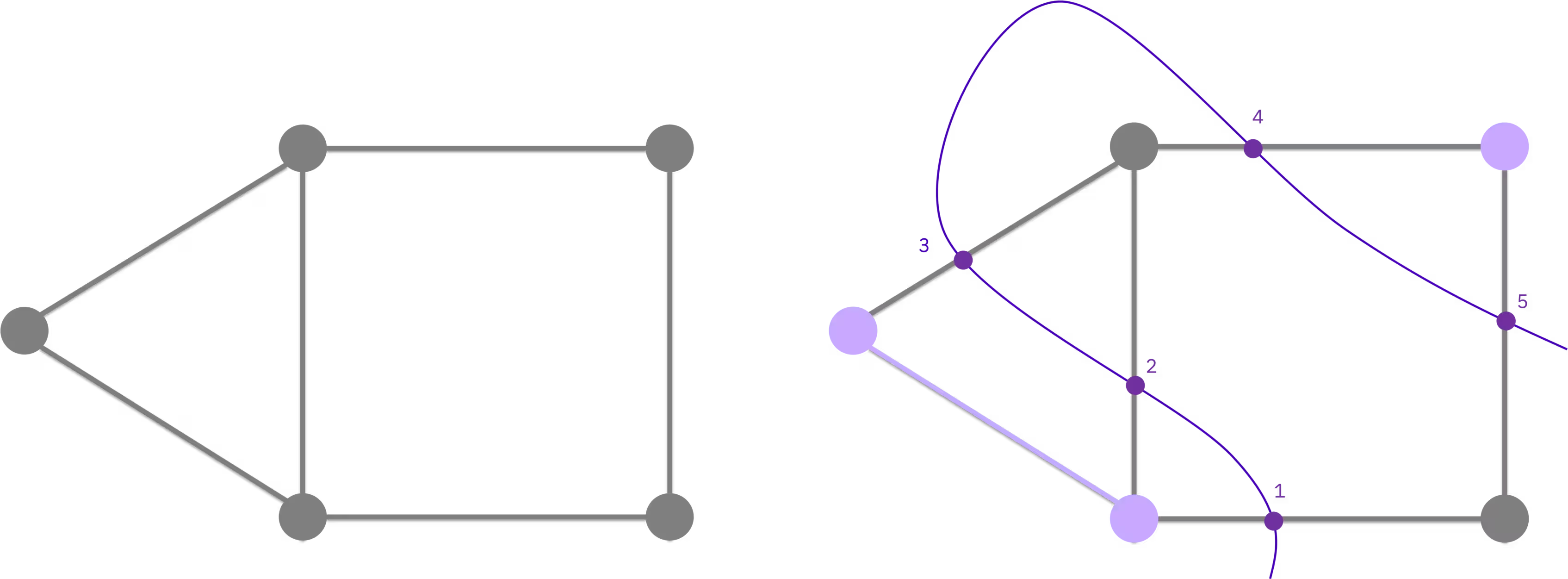
Det Minimum von $f(x)$ is in dem Fall erreicht, wenn die Zahl der vom Schnitt durchquerten Kanten maximal is. Wie du siehst, hat det noch nüscht mit Quantencomputing zu tun. Du musst dit Problem in'ne Form umformulieren, die 'n Quantencomputer verstehen kann. Initialisier dein Problem, indem du 'n Graphen mit $n=5$ Knoten erstellst.

n = 5

graph = rx.PyGraph()
graph.add_nodes_from(np.arange(0, n, 1))
edge_list = [
    (0, 1, 1.0),
    (0, 2, 1.0),
    (0, 4, 1.0),
    (1, 2, 1.0),
    (2, 3, 1.0),
    (3, 4, 1.0),
]
graph.add_edges_from(edge_list)
draw_graph(graph, node_size=600, with_labels=True)

Schritt 1: Klassische Eingaben auf 'n Quantenproblem abbildn

Da erste Schritt vom Muster is, det klassische Problem (den Graphen) auf Quanten-Schaltkreise un Operatoren abzubildn. Dafür gibt's drei Hauptschritte:

1. Eine Reihe von mathematischen Umformulierungen nutzen, um dat Problem in die Notation der Quadratic Unconstrained Binary Optimization (QUBO) zu bringen.
2. Det Optimierungsproblem als 'n Hamiltonian umschreiben, dessen Grundzustand der Lösung entspricht, die die Kostenfunktion minimiert.
3. Einen Quantenschaltkreis erstellen, der den Grundzustand von dem Hamiltonian durch 'n Prozess ähnlich wie Quantum Annealing vorbereitet.

Hinweis: Beim QAOA-Verfahren willste letztlich 'n Operator (Hamiltonian) haben, der die Kostenfunktion von unsrem hybriden Algorithmus darstellt, sowie 'n parametrisierten Schaltkreis (Ansatz), der Quantenzustände mit Kandidatenlösungen für dat Problem darstellt. Du kannst dann aus diesen Kandidatenzuständen sampln un sie mit da Kostenfunktion bewerten.

Graph → Optimierungsproblem

Da erste Schritt beim Abbilden is 'ne Notation­sumstellung. Hier wird det Problem in QUBO-Notation ausjedrückt:

$$\min_{x\in \{0, 1\}^n}x^T Q x,$$

wobei $Q$ 'ne $n\times n$-Matrix aus reellen Zahlen is, $n$ da Anzahl der Knoten in deim Graphen entspricht, $x$ da oben eingeführte Vektor aus binären Variablen is un $x^T$ die Transponierte von $x$ bezeichnet.

Maximize
 -2*x_0*x_1 - 2*x_0*x_2 - 2*x_0*x_4 - 2*x_1*x_2 - 2*x_2*x_3 - 2*x_3*x_4 + 3*x_0
 + 2*x_1 + 3*x_2 + 2*x_3 + 2*x_4

Subject to
  No constraints

  Binary variables (5)
    x_0 x_1 x_2 x_3 x_4

Optimierungsproblem → Hamiltonian

Det QUBO-Problem lässt sich dann als Hamiltonian umformulieren (also als Matrix, die die Energie eines Systems darstellt):

$$H_C=\sum_{ij}Q_{ij}Z_iZ_j + \sum_i b_iZ_i.$$

Umformulierungsschritte vom QAOA-Problem zum Hamiltonian

Um zu zeigen, wie sich det QAOA-Problem so umschreiben lässt, ersetzt man zunächst die binären Variablen $x_i$ durch 'ne neue Menge von Variablen $z_i\in\{-1, 1\}$ gemäß

$$x_i = \frac{1-z_i}{2}.$$

Hier siehste, datt wenn $x_i$ gleich $0$ ist, dann muss $z_i$ gleich $1$ sein. Wenn die $x_i$'s durch die $z_i$'s im Optimierungsproblem ($x^TQx$) ersetzt werden, ergibt sich 'ne äquivalente Formulierung.

$$x^TQx=\sum_{ij}Q_{ij}x_ix_j \\ =\frac{1}{4}\sum_{ij}Q_{ij}(1-z_i)(1-z_j) \\=\frac{1}{4}\sum_{ij}Q_{ij}z_iz_j-\frac{1}{4}\sum_{ij}(Q_{ij}+Q_{ji})z_i + \frac{n^2}{4}.$$

Wenn wir jetzt $b_i=-\sum_{j}(Q_{ij}+Q_{ji})$ definieren, den Vorfaktor rausnehmen un den konstanten Term $n^2$ weglassen, kommt man zu den zwei äquivalenten Formulierungen von demselbn Optimierungsproblem:

$$\min_{x\in\{0,1\}^n} x^TQx\Longleftrightarrow \min_{z\in\{-1,1\}^n}z^TQz + b^Tz$$

Hier hängt $b$ von $Q$ ab. Beachte, datt wir für $z^TQz + b^Tz$ den Faktor 1/4 un den konstanten Offset $n^2$ weggelassen haben, da die keene Rolle bei da Optimierung spieln.

Um jetzt 'ne Quantenformulierung vom Problem zu kriegen, befördert man die $z_i$-Variablen zu 'ner Pauli-$Z$-Matrix, also 'ner $2\times 2$-Matrix der Form

$$Z_i = \begin{pmatrix}1 & 0 \\ 0 & -1\end{pmatrix}.$$

Wenn man diese Matrizen in det oben stehende Optimierungsproblem einsetzt, ergibt sich folgender Hamiltonian:

$$H_C=\sum_{ij}Q_{ij}Z_iZ_j + \sum_i b_iZ_i.$$

Denk außadem daran, datt die $Z$-Matrizen in den Rechenraum vom Quantencomputer eingebettet sind, also in 'n Hilbertraum der Größe $2^n\times 2^n$. Daher solltest du Terme wie $Z_iZ_j$ als Tensorprodukt $Z_i\otimes Z_j$ im $2^n\times 2^n$-Hilbertraum verstehen. Bei 'nem Problem mit fünf Entscheidungsvariablen bedeutet zum Beispiel $Z_1Z_3$ genau $I\otimes Z_3\otimes I\otimes Z_1\otimes I$, wobei $I$ die $2\times 2$-Einheitsmatrix is.

Dieser Hamiltonian heißt Kostenfunktions-Hamiltonian. Er hat die Eigenschaft, datt sein Grundzustand der Lösung entspricht, die die Kostenfunktion $f(x)$ minimiert. Um dein Optimierungsproblem zu lösen, musste also jetzt den Grundzustand von $H_C$ (oder 'n Zustand mit hoher Überlappung damit) auf dem Quantencomputer vorbereiten. Wenn du aus diesem Zustand samplst, kriegste mit hoher Wahrscheinlichkeit die Lösung von $\min~f(x)$. Betrachten wa jetzt den Hamiltonian $H_C$ für det Max-Cut-Problem. Jeder Knoten des Graphen wird mit 'nem Qubit im Zustand $|0\rangle$ oder $|1\rangle$ verknüpft, wobei da Wert die Gruppe angibt, zu der der Knoten gehört. Det Ziel ist, die Zahl der Kanten $(v_1, v_2)$ zu maximieren, für die $v_1 = |0\rangle$ un $v_2 = |1\rangle$ gilt, oder umgekehrt. Wenn wir dem $Z$-Operator mit jedem Qubit verknüpfen, wobei

$$Z|0\rangle = |0\rangle \qquad Z|1\rangle = -|1\rangle$$

dann gehört 'ne Kante $(v_1, v_2)$ zum Schnitt, wenn da Eigenwert von $(Z_1|v_1\rangle) \cdot (Z_2|v_2\rangle) = -1$ is; also wenn die Qubits für $v_1$ un $v_2$ unterschiedlich sind. Genauso gehört $(v_1, v_2)$ nicht zum Schnitt, wenn da Eigenwert von $(Z_1|v_1\rangle) \cdot (Z_2|v_2\rangle) = 1$ is. Wichtig is dabei nicht da genaue Zustand des Qubits für jeden Knoten, sondern nur ob die Zustände über 'ne Kante gleich sind oder nicht. Det Max-Cut-Problem verlangt, 'ne Zuweisung der Qubits zu den Knoten zu finden, so datt da Eigenwert des folgenden Hamiltonians minimiert wird:

$$H_C = \sum_{(i,j) \in e} Q_{ij} \cdot Z_i Z_j.$$

Also gilt $b_i = 0$ für alle $i$ beim Max-Cut-Problem. Da Wert von $Q_{ij}$ gibt det Gewicht der Kante an. In diesem Tutorial betrachten wa 'n ungewichteten Graphen, also $Q_{ij} = 1.0$ für alle $i, j$.

def build_max_cut_paulis(
    graph: rx.PyGraph,
) -> list[tuple[str, list[int], float]]:
    """Convert the graph to Pauli list.

    This function does the inverse of `build_max_cut_graph`
    """
    pauli_list = []
    for edge in list(graph.edge_list()):
        weight = graph.get_edge_data(edge[0], edge[1])
        pauli_list.append(("ZZ", [edge[0], edge[1]], weight))
    return pauli_list


max_cut_paulis = build_max_cut_paulis(graph)
cost_hamiltonian = SparsePauliOp.from_sparse_list(max_cut_paulis, n)
print("Cost Function Hamiltonian:", cost_hamiltonian)

Cost Function Hamiltonian: SparsePauliOp(['IIIZZ', 'IIZIZ', 'ZIIIZ', 'IIZZI', 'IZZII', 'ZZIII'],
              coeffs=[1.+0.j, 1.+0.j, 1.+0.j, 1.+0.j, 1.+0.j, 1.+0.j])

Hamiltonian → Quantenschaltkreis

Da Hamiltonian $H_C$ enthält die Quantendefinition von deim Problem. Jetzt kannste 'n Quantenschaltkreis erstellen, der dabei hilft, gute Lösungen vom Quantencomputer zu sampln. Da QAOA orientiert sich am Quantum Annealing un wendet abwechselnde Schichten von Operatoren im Quantenschaltkreis an.

Die Grundidee is, in dem Grundzustand eines bekannten Systems zu startn, $H^{\otimes n}|0\rangle$ wie oben beschrieben, un dann det System in den Grundzustand vom Kostenoperator zu steuern, an dem du interessiert bist. Det passiert durch Anwenden der Operatoren $\exp\{-i\gamma_k H_C\}$ un $\exp\{-i\beta_k H_m\}$ mit den Winkeln $\gamma_1,...,\gamma_p$ un $\beta_1,...,\beta_p~$.

Da Quantenschaltkreis, den du generierst, is parametrisiert durch $\gamma_i$ un $\beta_i$, also kannste verschiedene Werte ausprobieren un aus dem resultierenden Zustand sampln.

In dem Fall probierste 'n Beispiel mit einer QAOA-Schicht mit zwei Parametern: $\gamma_1$ un $\beta_1$.

circuit = QAOAAnsatz(cost_operator=cost_hamiltonian, reps=2)
circuit.measure_all()

circuit.draw("mpl")

circuit.parameters

 ParameterView([ParameterVectorElement(β[0]), ParameterVectorElement(β[1]), ParameterVectorElement(γ[0]), ParameterVectorElement(γ[1])])

Schritt 2: Problem für die Quantenhardware-Ausführung optimieren

Da oben stehende Schaltkreis enthält 'ne Reihe von Abstraktionen, die nützlich für det Nachdenken über Quantenalgorithmen sind, aber nicht auf der Hardware laufn können. Um uff'm QPU ausjeführt wern zu können, muss der Schaltkreis 'ne Reihe von Operationen durchlaufn, die den Transpilation- oder Schaltkreisoptimierungs-Schritt vom Muster ausmahen.

Die Qiskit-Bibliothek bietet 'ne Reihe von Transpilations-Passes, die 'ne breite Palette von Schaltkreistransformationen abdecken. Du musst sicherstellen, datt dein Schaltkreis für deinen Zweck optimiert is.

Die Transpilation umfasst in der Regel mehrere Schritte, zum Beispiel:

• Initiales Mapping der Qubits im Schaltkreis (wie Entscheidungsvariablen) auf physikalische Qubits auf dem Gerät.
• Entrolllung der Anweisungen im Quantenschaltkreis in hardware-native Anweisungen, die der Backend versteht.
• Routing von Qubits im Schaltkreis, die miteinander interagieren, auf benachbarte physikalische Qubits.
• Fehlerunterdrückung durch Hinzufügen von Einzel-Qubit-Gates zur Rauschunterdrückung mit dynamischem Entkoppeln.

Mehr Infos zur Transpilation findst du in unsrer Dokumentation.

Da folgende Code transformiert und optimiert den abstrakten Schaltkreis in 'n Format, det zur Ausführung auf einem der üba die Cloud zugänglichen Geräte mit dem Qiskit IBM Runtime Service bereit is.

service = QiskitRuntimeService()
backend = service.least_busy(
    operational=True, simulator=False, min_num_qubits=127
)
print(backend)

# Create pass manager for transpilation
pm = generate_preset_pass_manager(optimization_level=3, backend=backend)

candidate_circuit = pm.run(circuit)
candidate_circuit.draw("mpl", fold=False, idle_wires=False)

<IBMBackend('test_heron_pok_1')>

Schritt 3: Ausführung mit Qiskit-Primitiven

Beim QAOA-Workflow werden die optimalen QAOA-Parameter in 'ner iterativen Optimierungsschleife gefunden, die 'ne Reihe von Schaltkreisauswertungen ausführt un 'n klassischen Optimierer nutzt, um die optimalen Parameter $\beta_k$ un $\gamma_k$ zu finden. Diese Ausführungsschleife läuft folgendermaßen ab:

1. Anfangsparameter definieren
2. 'ne neue Session instantiieren, die die Optimierungsschleife un das Primitive zum Sampln des Schaltkreises enthält
3. Sobald 'n optimaler Parametersatz gefunden wurde, den Schaltkreis ein letztes Mal ausführen, um 'ne finale Verteilung zu erhalten, die im Nachbearbeitungsschritt genutzt wird.

Schaltkreis mit Anfangsparametern definieren

Wir startn mit beliebig gewählten Parametern.

initial_gamma = np.pi
initial_beta = np.pi / 2
init_params = [initial_beta, initial_beta, initial_gamma, initial_gamma]

Backend un Ausführungsprimitiv definieren

Nutz die Qiskit Runtime-Primitive, um mit IBM®-Backends zu interagieren. Die beiden Primitive sind Sampler un Estimator, un die Wahl hängt davon ab, welche Art von Messung du auf dem Quantencomputer durchführn willst. Für die Minimierung von $H_C$ nimmst du den Estimator, da die Messung der Kostenfunktion einfach da Erwartungswert $\langle H_C \rangle$ is.

Ausführen

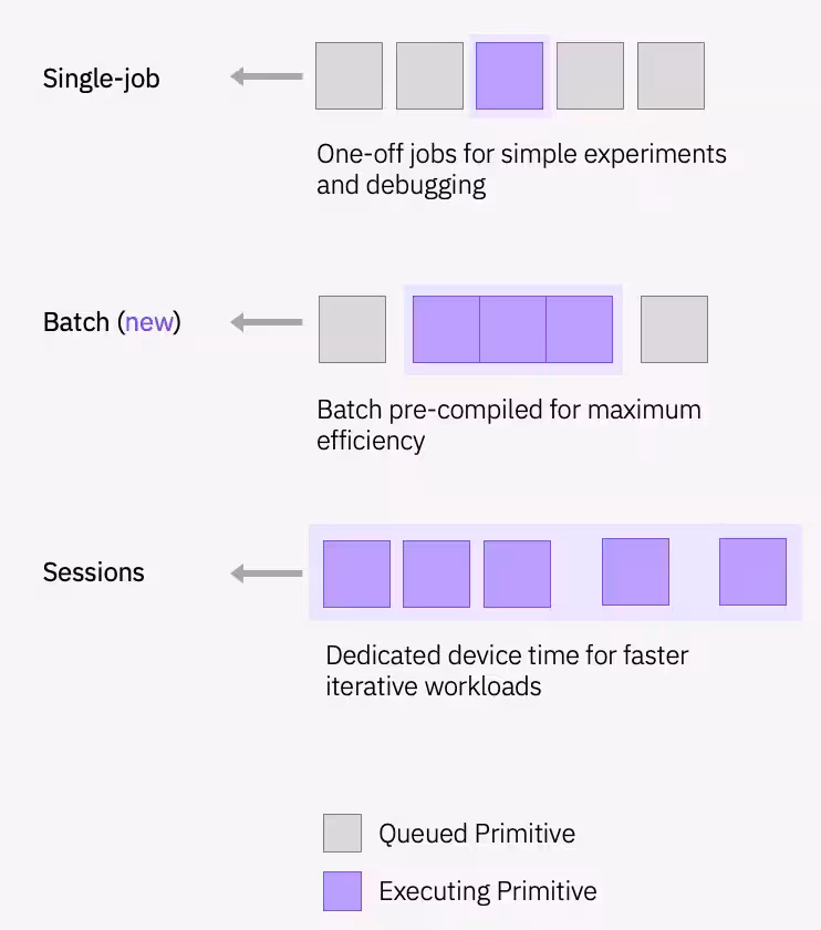
Die Primitive bieten 'ne Vielzahl von Ausführungsmodi, um Workloads auf Quantengeräten einzuplanen, un 'n QAOA-Workflow läuft iterativ in 'ner Session.

Du kannst die sampler-basierte Kostenfunktion in die SciPy-Minimierungsroutine einbaun, um die optimalen Parameter zu finden.

def cost_func_estimator(params, ansatz, hamiltonian, estimator):
    # transform the observable defined on virtual qubits to
    # an observable defined on all physical qubits
    isa_hamiltonian = hamiltonian.apply_layout(ansatz.layout)

    pub = (ansatz, isa_hamiltonian, params)
    job = estimator.run([pub])

    results = job.result()[0]
    cost = results.data.evs

    objective_func_vals.append(cost)

    return cost

objective_func_vals = []  # Global variable
with Session(backend=backend) as session:
    # If using qiskit-ibm-runtime<0.24.0, change `mode=` to `session=`
    estimator = Estimator(mode=session)
    estimator.options.default_shots = 1000

    # Set simple error suppression/mitigation options
    estimator.options.dynamical_decoupling.enable = True
    estimator.options.dynamical_decoupling.sequence_type = "XY4"
    estimator.options.twirling.enable_gates = True
    estimator.options.twirling.num_randomizations = "auto"

    result = minimize(
        cost_func_estimator,
        init_params,
        args=(candidate_circuit, cost_hamiltonian, estimator),
        method="COBYLA",
        tol=1e-2,
    )
    print(result)

message: Return from COBYLA because the trust region radius reaches its lower bound.
 success: True
  status: 0
     fun: -1.6295230263157894
       x: [ 1.530e+00  1.439e+00  4.071e+00  4.434e+00]
    nfev: 26
   maxcv: 0.0

Da Optimierer hat et geschafft, die Kosten zu reduzieren un bessere Parameter für den Schaltkreis zu finden.

plt.figure(figsize=(12, 6))
plt.plot(objective_func_vals)
plt.xlabel("Iteration")
plt.ylabel("Cost")
plt.show()

Wenn du die optimalen Parameter für den Schaltkreis gefunden hast, kannste die Parameter zuweisen un die finale Verteilung mit den optimierten Parametern sampln. Hier kommt det Sampler-Primitiv zum Einsatz, weil die Wahrscheinlichkeitsverteilung von Bitstring-Messungen dem optimalen Schnitt des Graphen entspricht.

Hinweis: Det bedeutet, 'n Quantenzustand $\psi$ im Rechner vorzubereiten un dann zu messen. 'ne Messung bringt den Zustand in 'n einzelnen Berechnungsbasis-Zustand zum Einsatz – zum Beispiel 010101110000... – der 'ner Kandidatenlösung $x$ für unser ursprüngliches Optimierungsproblem entspricht ($\max f(x)$ oder $\min f(x)$, je nach Aufgabe).

optimized_circuit = candidate_circuit.assign_parameters(result.x)
optimized_circuit.draw("mpl", fold=False, idle_wires=False)

# If using qiskit-ibm-runtime<0.24.0, change `mode=` to `backend=`
sampler = Sampler(mode=backend)
sampler.options.default_shots = 10000

# Set simple error suppression/mitigation options
sampler.options.dynamical_decoupling.enable = True
sampler.options.dynamical_decoupling.sequence_type = "XY4"
sampler.options.twirling.enable_gates = True
sampler.options.twirling.num_randomizations = "auto"

pub = (optimized_circuit,)
job = sampler.run([pub], shots=int(1e4))
counts_int = job.result()[0].data.meas.get_int_counts()
counts_bin = job.result()[0].data.meas.get_counts()
shots = sum(counts_int.values())
final_distribution_int = {key: val / shots for key, val in counts_int.items()}
final_distribution_bin = {key: val / shots for key, val in counts_bin.items()}
print(final_distribution_int)

{28: 0.0328, 11: 0.0343, 2: 0.0296, 25: 0.0308, 16: 0.0303, 27: 0.0302, 13: 0.0323, 7: 0.0312, 4: 0.0296, 9: 0.0295, 26: 0.0321, 30: 0.031, 23: 0.0324, 31: 0.0303, 21: 0.0335, 15: 0.0317, 12: 0.0309, 29: 0.0297, 3: 0.0313, 5: 0.0312, 6: 0.0274, 10: 0.0329, 22: 0.0353, 0: 0.0315, 20: 0.0326, 8: 0.0322, 14: 0.0306, 17: 0.0295, 18: 0.0279, 1: 0.0325, 24: 0.0334, 19: 0.0295}

Schritt 4: Nachbearbeitung un Rückgabe des Ergebnisses im gewünschten klassischen Format

Da Nachbearbeitungsschritt interpretiert die Sampling-Ausgabe, um 'ne Lösung für dein ursprüngliches Problem zurückzujeben. In dem Fall interessierste dich für den Bitstring mit der höchsten Wahrscheinlichkeit, denn der bestimmt den optimalen Schnitt. Die Symmetrien in dem Problem erlaubn vier mögliche Lösungen, un da Sampling-Prozess gibt 'ne davon mit 'ner leicht höheren Wahrscheinlichkeit zurück. In da unten plottn Verteilung siehste aber, datt vier der Bitstrings deutlich wahrscheinlicher sind als der Rest.

# auxiliary functions to sample most likely bitstring
def to_bitstring(integer, num_bits):
    result = np.binary_repr(integer, width=num_bits)
    return [int(digit) for digit in result]

keys = list(final_distribution_int.keys())
values = list(final_distribution_int.values())
most_likely = keys[np.argmax(np.abs(values))]
most_likely_bitstring = to_bitstring(most_likely, len(graph))
most_likely_bitstring.reverse()

print("Result bitstring:", most_likely_bitstring)

Result bitstring: [0, 1, 1, 0, 1]

matplotlib.rcParams.update({"font.size": 10})
final_bits = final_distribution_bin
values = np.abs(list(final_bits.values()))
top_4_values = sorted(values, reverse=True)[:4]
positions = []
for value in top_4_values:
    positions.append(np.where(values == value)[0])
fig = plt.figure(figsize=(11, 6))
ax = fig.add_subplot(1, 1, 1)
plt.xticks(rotation=45)
plt.title("Result Distribution")
plt.xlabel("Bitstrings (reversed)")
plt.ylabel("Probability")
ax.bar(list(final_bits.keys()), list(final_bits.values()), color="tab:grey")
for p in positions:
    ax.get_children()[int(p[0])].set_color("tab:purple")
plt.show()

Besten Schnitt visualisieren

Vom optimalen Bitstring aus kannste dann diesen Schnitt im ursprünglichen Graphen visualisieren.

# auxiliary function to plot graphs
def plot_result(G, x):
    colors = ["tab:grey" if i == 0 else "tab:purple" for i in x]
    pos, _default_axes = rx.spring_layout(G), plt.axes(frameon=True)
    rx.visualization.mpl_draw(
        G, node_color=colors, node_size=100, alpha=0.8, pos=pos
    )

plot_result(graph, most_likely_bitstring)

Un jetzt berechnste den Wert des Schnitts:

def evaluate_sample(x: Sequence[int], graph: rx.PyGraph) -> float:
    assert len(x) == len(
        list(graph.nodes())
    ), "The length of x must coincide with the number of nodes in the graph."
    return sum(
        x[u] * (1 - x[v]) + x[v] * (1 - x[u])
        for u, v in list(graph.edge_list())
    )

cut_value = evaluate_sample(most_likely_bitstring, graph)
print("The value of the cut is:", cut_value)

The value of the cut is: 5

Teil II. Janz groß skaln!

Du hast Zugang zu vielen Geräten mit üba 100 Qubits uff da IBM Quantum® Platform. Such dir eins aus, um Max-Cut auf 'nem gewichteten Graphen mit 100 Knoten zu lösen. Dit is 'n Problem im "Utility-Maßstab". Die Schritte zum Aufbau vom Workflow sind dieselben wie oben, nur mit 'nem viel größeren Graphen.

n = 100  # Number of nodes in graph
graph_100 = rx.PyGraph()
graph_100.add_nodes_from(np.arange(0, n, 1))
elist = []
for edge in backend.coupling_map:
    if edge[0] < n and edge[1] < n:
        elist.append((edge[0], edge[1], 1.0))
graph_100.add_edges_from(elist)
draw_graph(graph_100, node_size=200, with_labels=True, width=1)

Schritt 1: Klassische Eingaben auf 'n Quantenproblem abbildn

Graph → Hamiltonian

Konvertier zuerst den Graphen, den du lösen willst, direkt in 'n Hamiltonian, der für QAOA geeignet is.

max_cut_paulis_100 = build_max_cut_paulis(graph_100)

cost_hamiltonian_100 = SparsePauliOp.from_sparse_list(max_cut_paulis_100, 100)
print("Cost Function Hamiltonian:", cost_hamiltonian_100)

Cost Function Hamiltonian: SparsePauliOp(['IIIIIIIIIIIIIIIIIIIIIIIIIIIIIIIIIIIIIIIIIIIIIIIIIIIIIIIIIIIIIIIIIIIIIIIIIIIIIIIIIIIIIIIIIIIIIIIIIIZZ', 'IIIIIIIIIIIIIIIIIIIIIIIIIIIIIIIIIIIIIIIIIIIIIIIIIIIIIIIIIIIIIIIIIIIIIIIIIIIIIIIIIIIIIIIIIIIIIIIIIIZZ', 'IIIIIIIIIIIIIIIIIIIIIIIIIIIIIIIIIIIIIIIIIIIIIIIIIIIIIIIIIIIIIIIIIIIIIIIIIIIIIIIIIIIIIIIIIIIIIIIIIZZI', 'IIIIIIIIIIIIIIIIIIIIIIIIIIIIIIIIIIIIIIIIIIIIIIIIIIIIIIIIIIIIIIIIIIIIIIIIIIIIIIIIIIIIIIIIIIIIIIIIIZZI', 'IIIIIIIIIIIIIIIIIIIIIIIIIIIIIIIIIIIIIIIIIIIIIIIIIIIIIIIIIIIIIIIIIIIIIIIIIIIIIIIIIIIIIIIIIIIIIIIIZZII', 'IIIIIIIIIIIIIIIIIIIIIIIIIIIIIIIIIIIIIIIIIIIIIIIIIIIIIIIIIIIIIIIIIIIIIIIIIIIIIIIIIIIIIIIIIIIIIIIIZZII', 'IIIIIIIIIIIIIIIIIIIIIIIIIIIIIIIIIIIIIIIIIIIIIIIIIIIIIIIIIIIIIIIIIIIIIIIIIIIIIIIIIIIIIIIIIIIIIIIZZIII', 'IIIIIIIIIIIIIIIIIIIIIIIIIIIIIIIIIIIIIIIIIIIIIIIIIIIIIIIIIIIIIIIIIIIIIIIIIIIIIIIIIIIZIIIIIIIIIIIIZIII', 'IIIIIIIIIIIIIIIIIIIIIIIIIIIIIIIIIIIIIIIIIIIIIIIIIIIIIIIIIIIIIIIIIIIIIIIIIIIIIIIIIIIIIIIIIIIIIIIZZIII', 'IIIIIIIIIIIIIIIIIIIIIIIIIIIIIIIIIIIIIIIIIIIIIIIIIIIIIIIIIIIIIIIIIIIIIIIIIIIIIIIIIIIIIIIIIIIIIIZZIIII', 'IIIIIIIIIIIIIIIIIIIIIIIIIIIIIIIIIIIIIIIIIIIIIIIIIIIIIIIIIIIIIIIIIIIIIIIIIIIIIIIIIIIIIIIIIIIIIIZZIIII', 'IIIIIIIIIIIIIIIIIIIIIIIIIIIIIIIIIIIIIIIIIIIIIIIIIIIIIIIIIIIIIIIIIIIIIIIIIIIIIIIIIIIIIIIIIIIIIZZIIIII', 'IIIIIIIIIIIIIIIIIIIIIIIIIIIIIIIIIIIIIIIIIIIIIIIIIIIIIIIIIIIIIIIIIIIIIIIIIIIIIIIIIIIIIIIIIIIIIZZIIIII', 'IIIIIIIIIIIIIIIIIIIIIIIIIIIIIIIIIIIIIIIIIIIIIIIIIIIIIIIIIIIIIIIIIIIIIIIIIIIIIIIIIIIIIIIIIIIIZZIIIIII', 'IIIIIIIIIIIIIIIIIIIIIIIIIIIIIIIIIIIIIIIIIIIIIIIIIIIIIIIIIIIIIIIIIIIIIIIIIIIIIIIIIIIIIIIIIIIIZZIIIIII', 'IIIIIIIIIIIIIIIIIIIIIIIIIIIIIIIIIIIIIIIIIIIIIIIIIIIIIIIIIIIIIIIIIIIIIIIIIIIIIIIIIIIIIIIIIIIZZIIIIIII', 'IIIIIIIIIIIIIIIIIIIIIIIIIIIIIIIIIIIIIIIIIIIIIIIIIIIIIIIIIIIIIIIIIIIIIIIIIIIIIIIIIIZIIIIIIIIIZIIIIIII', 'IIIIIIIIIIIIIIIIIIIIIIIIIIIIIIIIIIIIIIIIIIIIIIIIIIIIIIIIIIIIIIIIIIIIIIIIIIIIIIIIIIIIIIIIIIIZZIIIIIII', 'IIIIIIIIIIIIIIIIIIIIIIIIIIIIIIIIIIIIIIIIIIIIIIIIIIIIIIIIIIIIIIIIIIIIIIIIIIIIIIIIIIIIIIIIIIZZIIIIIIII', 'IIIIIIIIIIIIIIIIIIIIIIIIIIIIIIIIIIIIIIIIIIIIIIIIIIIIIIIIIIIIIIIIIIIIIIIIIIIIIIIIIIIIIIIIIIZZIIIIIIII', 'IIIIIIIIIIIIIIIIIIIIIIIIIIIIIIIIIIIIIIIIIIIIIIIIIIIIIIIIIIIIIIIIIIIIIIIIIIIIIIIIIIIIIIIIIZZIIIIIIIII', 'IIIIIIIIIIIIIIIIIIIIIIIIIIIIIIIIIIIIIIIIIIIIIIIIIIIIIIIIIIIIIIIIIIIIIIIIIIIIIIIIIIIIIIIIIZZIIIIIIIII', 'IIIIIIIIIIIIIIIIIIIIIIIIIIIIIIIIIIIIIIIIIIIIIIIIIIIIIIIIIIIIIIIIIIIIIIIIIIIIIIIIIIIIIIIIZZIIIIIIIIII', 'IIIIIIIIIIIIIIIIIIIIIIIIIIIIIIIIIIIIIIIIIIIIIIIIIIIIIIIIIIIIIIIIIIIIIIIIIIIIIIIIIIIIIIIIZZIIIIIIIIII', 'IIIIIIIIIIIIIIIIIIIIIIIIIIIIIIIIIIIIIIIIIIIIIIIIIIIIIIIIIIIIIIIIIIIIIIIIIIIIIIIIIIIIIIIZZIIIIIIIIIII', 'IIIIIIIIIIIIIIIIIIIIIIIIIIIIIIIIIIIIIIIIIIIIIIIIIIIIIIIIIIIIIIIIIIIIIIIIIIIIIIIIIZIIIIIIZIIIIIIIIIII', 'IIIIIIIIIIIIIIIIIIIIIIIIIIIIIIIIIIIIIIIIIIIIIIIIIIIIIIIIIIIIIIIIIIIIIIIIIIIIIIIIIIIIIIIZZIIIIIIIIIII', 'IIIIIIIIIIIIIIIIIIIIIIIIIIIIIIIIIIIIIIIIIIIIIIIIIIIIIIIIIIIIIIIIIIIIIIIIIIIIIIIIIIIIIIZZIIIIIIIIIIII', 'IIIIIIIIIIIIIIIIIIIIIIIIIIIIIIIIIIIIIIIIIIIIIIIIIIIIIIIIIIIIIIIIIIIIIIIIIIIIIIIIIIIIIIZZIIIIIIIIIIII', 'IIIIIIIIIIIIIIIIIIIIIIIIIIIIIIIIIIIIIIIIIIIIIIIIIIIIIIIIIIIIIIIIIIIIIIIIIIIIIIIIIIIIIZZIIIIIIIIIIIII', 'IIIIIIIIIIIIIIIIIIIIIIIIIIIIIIIIIIIIIIIIIIIIIIIIIIIIIIIIIIIIIIIIIIIIIIIIIIIIIIIIIIIIIZZIIIIIIIIIIIII', 'IIIIIIIIIIIIIIIIIIIIIIIIIIIIIIIIIIIIIIIIIIIIIIIIIIIIIIIIIIIIIIIIIIIIIIIIIIIIIIIIIIIIZZIIIIIIIIIIIIII', 'IIIIIIIIIIIIIIIIIIIIIIIIIIIIIIIIIIIIIIIIIIIIIIIIIIIIIIIIIIIIIIIIIIIIIIIIIIIIIIIIIIIIZZIIIIIIIIIIIIII', 'IIIIIIIIIIIIIIIIIIIIIIIIIIIIIIIIIIIIIIIIIIIIIIIIIIIIIIIIIIIIIIIIIIIIIIIIIIIIIIIIZIIIZIIIIIIIIIIIIIII', 'IIIIIIIIIIIIIIIIIIIIIIIIIIIIIIIIIIIIIIIIIIIIIIIIIIIIIIIIIIIIIIIIIIIIIIIIIIIIIIIIIIIZIIIIIIIIIIIIZIII', 'IIIIIIIIIIIIIIIIIIIIIIIIIIIIIIIIIIIIIIIIIIIIIIIIIIIIIIIIIIIIIIIIIIIIIIIIIIIIZIIIIIIZIIIIIIIIIIIIIIII', 'IIIIIIIIIIIIIIIIIIIIIIIIIIIIIIIIIIIIIIIIIIIIIIIIIIIIIIIIIIIIIIIIIIIIIIIIIIIIIIIIIIZIIIIIIIIIZIIIIIII', 'IIIIIIIIIIIIIIIIIIIIIIIIIIIIIIIIIIIIIIIIIIIIIIIIIIIIIIIIIIIIIIIIIIIIIIIIZIIIIIIIIIZIIIIIIIIIIIIIIIII', 'IIIIIIIIIIIIIIIIIIIIIIIIIIIIIIIIIIIIIIIIIIIIIIIIIIIIIIIIIIIIIIIIIIIIIIIIIIIIIIIIIZIIIIIIZIIIIIIIIIII', 'IIIIIIIIIIIIIIIIIIIIIIIIIIIIIIIIIIIIIIIIIIIIIIIIIIIIIIIIIIIIIIIIIIIIZIIIIIIIIIIIIZIIIIIIIIIIIIIIIIII', 'IIIIIIIIIIIIIIIIIIIIIIIIIIIIIIIIIIIIIIIIIIIIIIIIIIIIIIIIIIIIIIIIIIIIIIIIIIIIIIIIZIIIZIIIIIIIIIIIIIII', 'IIIIIIIIIIIIIIIIIIIIIIIIIIIIIIIIIIIIIIIIIIIIIIIIIIIIIIIIIIIIIIIIZIIIIIIIIIIIIIIIZIIIIIIIIIIIIIIIIIII', 'IIIIIIIIIIIIIIIIIIIIIIIIIIIIIIIIIIIIIIIIIIIIIIIIIIIIIIIIIIIIIIIIIIIIIIIIIIIIIIZZIIIIIIIIIIIIIIIIIIII', 'IIIIIIIIIIIIIIIIIIIIIIIIIIIIIIIIIIIIIIIIIIIIIIIIIIIIIIIIIIIIIIIIIIIIIIIIIIIIIIZZIIIIIIIIIIIIIIIIIIII', 'IIIIIIIIIIIIIIIIIIIIIIIIIIIIIIIIIIIIIIIIIIIIIIIIIIIIIIIIIIIIIIIIIIIIIIIIIIIIIZZIIIIIIIIIIIIIIIIIIIII', 'IIIIIIIIIIIIIIIIIIIIIIIIIIIIIIIIIIIIIIIIIIIIIIIIIIIIIIIIIIIIIIIZIIIIIIIIIIIIIIZIIIIIIIIIIIIIIIIIIIII', 'IIIIIIIIIIIIIIIIIIIIIIIIIIIIIIIIIIIIIIIIIIIIIIIIIIIIIIIIIIIIIIIIIIIIIIIIIIIIIZZIIIIIIIIIIIIIIIIIIIII', 'IIIIIIIIIIIIIIIIIIIIIIIIIIIIIIIIIIIIIIIIIIIIIIIIIIIIIIIIIIIIIIIIIIIIIIIIIIIIZZIIIIIIIIIIIIIIIIIIIIII', 'IIIIIIIIIIIIIIIIIIIIIIIIIIIIIIIIIIIIIIIIIIIIIIIIIIIIIIIIIIIIIIIIIIIIIIIIIIIIZIIIIIIZIIIIIIIIIIIIIIII', 'IIIIIIIIIIIIIIIIIIIIIIIIIIIIIIIIIIIIIIIIIIIIIIIIIIIIIIIIIIIIIIIIIIIIIIIIIIIIZZIIIIIIIIIIIIIIIIIIIIII', 'IIIIIIIIIIIIIIIIIIIIIIIIIIIIIIIIIIIIIIIIIIIIIIIIIIIIIIIIIIIIIIIIIIIIIIIIIIIZZIIIIIIIIIIIIIIIIIIIIIII', 'IIIIIIIIIIIIIIIIIIIIIIIIIIIIIIIIIIIIIIIIIIIIIIIIIIIIIIIIIIIIIIIIIIIIIIIIIIIZZIIIIIIIIIIIIIIIIIIIIIII', 'IIIIIIIIIIIIIIIIIIIIIIIIIIIIIIIIIIIIIIIIIIIIIIIIIIIIIIIIIIIIIIIIIIIIIIIIIIZZIIIIIIIIIIIIIIIIIIIIIIII', 'IIIIIIIIIIIIIIIIIIIIIIIIIIIIIIIIIIIIIIIIIIIIIIIIIIIIIIIIIIIIIIIIIIIIIIIIIIZZIIIIIIIIIIIIIIIIIIIIIIII', 'IIIIIIIIIIIIIIIIIIIIIIIIIIIIIIIIIIIIIIIIIIIIIIIIIIIIIIIIIIIIIIIIIIIIIIIIIZZIIIIIIIIIIIIIIIIIIIIIIIII', 'IIIIIIIIIIIIIIIIIIIIIIIIIIIIIIIIIIIIIIIIIIIIIIIIIIIIIIIIIIIIIIZIIIIIIIIIIIZIIIIIIIIIIIIIIIIIIIIIIIII', 'IIIIIIIIIIIIIIIIIIIIIIIIIIIIIIIIIIIIIIIIIIIIIIIIIIIIIIIIIIIIIIIIIIIIIIIIIZZIIIIIIIIIIIIIIIIIIIIIIIII', 'IIIIIIIIIIIIIIIIIIIIIIIIIIIIIIIIIIIIIIIIIIIIIIIIIIIIIIIIIIIIIIIIIIIIIIIIZZIIIIIIIIIIIIIIIIIIIIIIIIII', 'IIIIIIIIIIIIIIIIIIIIIIIIIIIIIIIIIIIIIIIIIIIIIIIIIIIIIIIIIIIIIIIIIIIIIIIIZIIIIIIIIIZIIIIIIIIIIIIIIIII', 'IIIIIIIIIIIIIIIIIIIIIIIIIIIIIIIIIIIIIIIIIIIIIIIIIIIIIIIIIIIIIIIIIIIIIIIIZZIIIIIIIIIIIIIIIIIIIIIIIIII', 'IIIIIIIIIIIIIIIIIIIIIIIIIIIIIIIIIIIIIIIIIIIIIIIIIIIIIIIIIIIIIIIIIIIIIIIZZIIIIIIIIIIIIIIIIIIIIIIIIIII', 'IIIIIIIIIIIIIIIIIIIIIIIIIIIIIIIIIIIIIIIIIIIIIIIIIIIIIIIIIIIIIIIIIIIIIIIZZIIIIIIIIIIIIIIIIIIIIIIIIIII', 'IIIIIIIIIIIIIIIIIIIIIIIIIIIIIIIIIIIIIIIIIIIIIIIIIIIIIIIIIIIIIIIIIIIIIIZZIIIIIIIIIIIIIIIIIIIIIIIIIIII', 'IIIIIIIIIIIIIIIIIIIIIIIIIIIIIIIIIIIIIIIIIIIIIIIIIIIIIIIIIIIIIIIIIIIIIIZZIIIIIIIIIIIIIIIIIIIIIIIIIIII', 'IIIIIIIIIIIIIIIIIIIIIIIIIIIIIIIIIIIIIIIIIIIIIIIIIIIIIIIIIIIIIIIIIIIIIZZIIIIIIIIIIIIIIIIIIIIIIIIIIIII', 'IIIIIIIIIIIIIIIIIIIIIIIIIIIIIIIIIIIIIIIIIIIIIIIIIIIIIIIIIIIIIZIIIIIIIIZIIIIIIIIIIIIIIIIIIIIIIIIIIIII', 'IIIIIIIIIIIIIIIIIIIIIIIIIIIIIIIIIIIIIIIIIIIIIIIIIIIIIIIIIIIIIIIIIIIIIZZIIIIIIIIIIIIIIIIIIIIIIIIIIIII', 'IIIIIIIIIIIIIIIIIIIIIIIIIIIIIIIIIIIIIIIIIIIIIIIIIIIIIIIIIIIIIIIIIIIIZZIIIIIIIIIIIIIIIIIIIIIIIIIIIIII', 'IIIIIIIIIIIIIIIIIIIIIIIIIIIIIIIIIIIIIIIIIIIIIIIIIIIIIIIIIIIIIIIIIIIIZIIIIIIIIIIIIZIIIIIIIIIIIIIIIIII', 'IIIIIIIIIIIIIIIIIIIIIIIIIIIIIIIIIIIIIIIIIIIIIIIIIIIIIIIIIIIIIIIIIIIIZZIIIIIIIIIIIIIIIIIIIIIIIIIIIIII', 'IIIIIIIIIIIIIIIIIIIIIIIIIIIIIIIIIIIIIIIIIIIIIIIIIIIIIIIIIIIIIIIIIIIZZIIIIIIIIIIIIIIIIIIIIIIIIIIIIIII', 'IIIIIIIIIIIIIIIIIIIIIIIIIIIIIIIIIIIIIIIIIIIIIIIIIIIIIIIIIIIIIIIIIIIZZIIIIIIIIIIIIIIIIIIIIIIIIIIIIIII', 'IIIIIIIIIIIIIIIIIIIIIIIIIIIIIIIIIIIIIIIIIIIIIIIIIIIIIIIIIIIIIIIIIIZZIIIIIIIIIIIIIIIIIIIIIIIIIIIIIIII', 'IIIIIIIIIIIIIIIIIIIIIIIIIIIIIIIIIIIIIIIIIIIIIIIIIIIIIIIIIIIIIIIIIIZZIIIIIIIIIIIIIIIIIIIIIIIIIIIIIIII', 'IIIIIIIIIIIIIIIIIIIIIIIIIIIIIIIIIIIIIIIIIIIIIIIIIIIIIIIIIIIIIIIIIZZIIIIIIIIIIIIIIIIIIIIIIIIIIIIIIIII', 'IIIIIIIIIIIIIIIIIIIIIIIIIIIIIIIIIIIIIIIIIIIIIIIIIIIIIIIIIIIIZIIIIIZIIIIIIIIIIIIIIIIIIIIIIIIIIIIIIIII', 'IIIIIIIIIIIIIIIIIIIIIIIIIIIIIIIIIIIIIIIIIIIIIIIIIIIIIIIIIIIIIIIIIZZIIIIIIIIIIIIIIIIIIIIIIIIIIIIIIIII', 'IIIIIIIIIIIIIIIIIIIIIIIIIIIIIIIIIIIIIIIIIIIIIIIIIIIIIIIIIIIIIIIIZZIIIIIIIIIIIIIIIIIIIIIIIIIIIIIIIIII', 'IIIIIIIIIIIIIIIIIIIIIIIIIIIIIIIIIIIIIIIIIIIIIIIIIIIIIIIIIIIIIIIIZIIIIIIIIIIIIIIIZIIIIIIIIIIIIIIIIIII', 'IIIIIIIIIIIIIIIIIIIIIIIIIIIIIIIIIIIIIIIIIIIIIIIIIIIIIIIIIIIIIIIIZZIIIIIIIIIIIIIIIIIIIIIIIIIIIIIIIIII', 'IIIIIIIIIIIIIIIIIIIIIIIIIIIIIIIIIIIIIIIIIIIIIIIIIIIIIIIIIIIIIIIZIIIIIIIIIIIIIIZIIIIIIIIIIIIIIIIIIIII', 'IIIIIIIIIIIIIIIIIIIIIIIIIIIIIIIIIIIIIIIIIIIIIIIIIIIIIIIIIIZIIIIZIIIIIIIIIIIIIIIIIIIIIIIIIIIIIIIIIIII', 'IIIIIIIIIIIIIIIIIIIIIIIIIIIIIIIIIIIIIIIIIIIIIIIIIIIIIIIIIIIIIIZIIIIIIIIIIIZIIIIIIIIIIIIIIIIIIIIIIIII', 'IIIIIIIIIIIIIIIIIIIIIIIIIIIIIIIIIIIIIIIIIIIIIIIIIIIIIIZIIIIIIIZIIIIIIIIIIIIIIIIIIIIIIIIIIIIIIIIIIIII', 'IIIIIIIIIIIIIIIIIIIIIIIIIIIIIIIIIIIIIIIIIIIIIIIIIIIIIIIIIIIIIZIIIIIIIIZIIIIIIIIIIIIIIIIIIIIIIIIIIIII', 'IIIIIIIIIIIIIIIIIIIIIIIIIIIIIIIIIIIIIIIIIIIIIIIIIIZIIIIIIIIIIZIIIIIIIIIIIIIIIIIIIIIIIIIIIIIIIIIIIIII', 'IIIIIIIIIIIIIIIIIIIIIIIIIIIIIIIIIIIIIIIIIIIIIIIIIIIIIIIIIIIIZIIIIIZIIIIIIIIIIIIIIIIIIIIIIIIIIIIIIIII', 'IIIIIIIIIIIIIIIIIIIIIIIIIIIIIIIIIIIIIIIIIIIIIIZIIIIIIIIIIIIIZIIIIIIIIIIIIIIIIIIIIIIIIIIIIIIIIIIIIIII', 'IIIIIIIIIIIIIIIIIIIIIIIIIIIIIIIIIIIIIIIIIIIIIIIIIIIIIIIIIIZZIIIIIIIIIIIIIIIIIIIIIIIIIIIIIIIIIIIIIIII', 'IIIIIIIIIIIIIIIIIIIIIIIIIIIIIIIIIIIIIIIIIIIIIIIIIIIIIIIIIIZIIIIZIIIIIIIIIIIIIIIIIIIIIIIIIIIIIIIIIIII', 'IIIIIIIIIIIIIIIIIIIIIIIIIIIIIIIIIIIIIIIIIIIIIIIIIIIIIIIIIIZZIIIIIIIIIIIIIIIIIIIIIIIIIIIIIIIIIIIIIIII', 'IIIIIIIIIIIIIIIIIIIIIIIIIIIIIIIIIIIIIIIIIIIIIIIIIIIIIIIIIZZIIIIIIIIIIIIIIIIIIIIIIIIIIIIIIIIIIIIIIIII', 'IIIIIIIIIIIIIIIIIIIIIIIIIIIIIIIIIIIIIIIIIIIIIIIIIIIIIIIIIZZIIIIIIIIIIIIIIIIIIIIIIIIIIIIIIIIIIIIIIIII', 'IIIIIIIIIIIIIIIIIIIIIIIIIIIIIIIIIIIIIIIIIIIIIIIIIIIIIIIIZZIIIIIIIIIIIIIIIIIIIIIIIIIIIIIIIIIIIIIIIIII', 'IIIIIIIIIIIIIIIIIIIIIIIIIIIIIIIIIIIIIIIIIIIIIIIIIIIIIIIIZZIIIIIIIIIIIIIIIIIIIIIIIIIIIIIIIIIIIIIIIIII', 'IIIIIIIIIIIIIIIIIIIIIIIIIIIIIIIIIIIIIIIIIIIIIIIIIIIIIIIZZIIIIIIIIIIIIIIIIIIIIIIIIIIIIIIIIIIIIIIIIIII', 'IIIIIIIIIIIIIIIIIIIIIIIIIIIIIIIIIIIIIIIIIIIZIIIIIIIIIIIIZIIIIIIIIIIIIIIIIIIIIIIIIIIIIIIIIIIIIIIIIIII', 'IIIIIIIIIIIIIIIIIIIIIIIIIIIIIIIIIIIIIIIIIIIIIIIIIIIIIIIZZIIIIIIIIIIIIIIIIIIIIIIIIIIIIIIIIIIIIIIIIIII', 'IIIIIIIIIIIIIIIIIIIIIIIIIIIIIIIIIIIIIIIIIIIIIIIIIIIIIIZZIIIIIIIIIIIIIIIIIIIIIIIIIIIIIIIIIIIIIIIIIIII', 'IIIIIIIIIIIIIIIIIIIIIIIIIIIIIIIIIIIIIIIIIIIIIIIIIIIIIIZIIIIIIIZIIIIIIIIIIIIIIIIIIIIIIIIIIIIIIIIIIIII', 'IIIIIIIIIIIIIIIIIIIIIIIIIIIIIIIIIIIIIIIIIIIIIIIIIIIIIIZZIIIIIIIIIIIIIIIIIIIIIIIIIIIIIIIIIIIIIIIIIIII', 'IIIIIIIIIIIIIIIIIIIIIIIIIIIIIIIIIIIIIIIIIIIIIIIIIIIIIZZIIIIIIIIIIIIIIIIIIIIIIIIIIIIIIIIIIIIIIIIIIIII', 'IIIIIIIIIIIIIIIIIIIIIIIIIIIIIIIIIIIIIIIIIIIIIIIIIIIIIZZIIIIIIIIIIIIIIIIIIIIIIIIIIIIIIIIIIIIIIIIIIIII', 'IIIIIIIIIIIIIIIIIIIIIIIIIIIIIIIIIIIIIIIIIIIIIIIIIIIIZZIIIIIIIIIIIIIIIIIIIIIIIIIIIIIIIIIIIIIIIIIIIIII', 'IIIIIIIIIIIIIIIIIIIIIIIIIIIIIIIIIIIIIIIIIIIIIIIIIIIIZZIIIIIIIIIIIIIIIIIIIIIIIIIIIIIIIIIIIIIIIIIIIIII', 'IIIIIIIIIIIIIIIIIIIIIIIIIIIIIIIIIIIIIIIIIIIIIIIIIIIZZIIIIIIIIIIIIIIIIIIIIIIIIIIIIIIIIIIIIIIIIIIIIIII', 'IIIIIIIIIIIIIIIIIIIIIIIIIIIIIIIIIIIIIIIIIIZIIIIIIIIIZIIIIIIIIIIIIIIIIIIIIIIIIIIIIIIIIIIIIIIIIIIIIIII', 'IIIIIIIIIIIIIIIIIIIIIIIIIIIIIIIIIIIIIIIIIIIIIIIIIIIZZIIIIIIIIIIIIIIIIIIIIIIIIIIIIIIIIIIIIIIIIIIIIIII', 'IIIIIIIIIIIIIIIIIIIIIIIIIIIIIIIIIIIIIIIIIIIIIIIIIIZZIIIIIIIIIIIIIIIIIIIIIIIIIIIIIIIIIIIIIIIIIIIIIIII', 'IIIIIIIIIIIIIIIIIIIIIIIIIIIIIIIIIIIIIIIIIIIIIIIIIIZIIIIIIIIIIZIIIIIIIIIIIIIIIIIIIIIIIIIIIIIIIIIIIIII', 'IIIIIIIIIIIIIIIIIIIIIIIIIIIIIIIIIIIIIIIIIIIIIIIIIIZZIIIIIIIIIIIIIIIIIIIIIIIIIIIIIIIIIIIIIIIIIIIIIIII', 'IIIIIIIIIIIIIIIIIIIIIIIIIIIIIIIIIIIIIIIIIIIIIIIIIZZIIIIIIIIIIIIIIIIIIIIIIIIIIIIIIIIIIIIIIIIIIIIIIIII', 'IIIIIIIIIIIIIIIIIIIIIIIIIIIIIIIIIIIIIIIIIIIIIIIIIZZIIIIIIIIIIIIIIIIIIIIIIIIIIIIIIIIIIIIIIIIIIIIIIIII', 'IIIIIIIIIIIIIIIIIIIIIIIIIIIIIIIIIIIIIIIIIIIIIIIIZZIIIIIIIIIIIIIIIIIIIIIIIIIIIIIIIIIIIIIIIIIIIIIIIIII', 'IIIIIIIIIIIIIIIIIIIIIIIIIIIIIIIIIIIIIIIIIIIIIIIIZZIIIIIIIIIIIIIIIIIIIIIIIIIIIIIIIIIIIIIIIIIIIIIIIIII', 'IIIIIIIIIIIIIIIIIIIIIIIIIIIIIIIIIIIIIIIIIIIIIIIZZIIIIIIIIIIIIIIIIIIIIIIIIIIIIIIIIIIIIIIIIIIIIIIIIIII', 'IIIIIIIIIIIIIIIIIIIIIIIIIIIIIIIIIIIIIIIIIZIIIIIIZIIIIIIIIIIIIIIIIIIIIIIIIIIIIIIIIIIIIIIIIIIIIIIIIIII', 'IIIIIIIIIIIIIIIIIIIIIIIIIIIIIIIIIIIIIIIIIIIIIIIZZIIIIIIIIIIIIIIIIIIIIIIIIIIIIIIIIIIIIIIIIIIIIIIIIIII', 'IIIIIIIIIIIIIIIIIIIIIIIIIIIIIIIIIIIIIIIIIIIIIIZZIIIIIIIIIIIIIIIIIIIIIIIIIIIIIIIIIIIIIIIIIIIIIIIIIIII', 'IIIIIIIIIIIIIIIIIIIIIIIIIIIIIIIIIIIIIIIIIIIIIIZIIIIIIIIIIIIIZIIIIIIIIIIIIIIIIIIIIIIIIIIIIIIIIIIIIIII', 'IIIIIIIIIIIIIIIIIIIIIIIIIIIIIIIIIIIIIIIIIIIIIIZZIIIIIIIIIIIIIIIIIIIIIIIIIIIIIIIIIIIIIIIIIIIIIIIIIIII', 'IIIIIIIIIIIIIIIIIIIIIIIIIIIIIIIIIIIIIIIIIIIIIZZIIIIIIIIIIIIIIIIIIIIIIIIIIIIIIIIIIIIIIIIIIIIIIIIIIIII', 'IIIIIIIIIIIIIIIIIIIIIIIIIIIIIIIIIIIIIIIIIIIIIZZIIIIIIIIIIIIIIIIIIIIIIIIIIIIIIIIIIIIIIIIIIIIIIIIIIIII', 'IIIIIIIIIIIIIIIIIIIIIIIIIIIIIIIIIIIIIIIIIIIIZZIIIIIIIIIIIIIIIIIIIIIIIIIIIIIIIIIIIIIIIIIIIIIIIIIIIIII', 'IIIIIIIIIIIIIIIIIIIIIIIIIIIIIIIIIIIIIIIIIIIIZZIIIIIIIIIIIIIIIIIIIIIIIIIIIIIIIIIIIIIIIIIIIIIIIIIIIIII', 'IIIIIIIIIIIIIIIIIIIIIIIIIIIIIIIIIIIIIIIIZIIIZIIIIIIIIIIIIIIIIIIIIIIIIIIIIIIIIIIIIIIIIIIIIIIIIIIIIIII', 'IIIIIIIIIIIIIIIIIIIIIIIIIIIIIIIIIIIIIIIIIIIZIIIIIIIIIIIIZIIIIIIIIIIIIIIIIIIIIIIIIIIIIIIIIIIIIIIIIIII', 'IIIIIIIIIIIIIIIIIIIIIIIIIIIIIIIIIIIIZIIIIIIZIIIIIIIIIIIIIIIIIIIIIIIIIIIIIIIIIIIIIIIIIIIIIIIIIIIIIIII', 'IIIIIIIIIIIIIIIIIIIIIIIIIIIIIIIIIIIIIIIIIIZIIIIIIIIIZIIIIIIIIIIIIIIIIIIIIIIIIIIIIIIIIIIIIIIIIIIIIIII', 'IIIIIIIIIIIIIIIIIIIIIIIIIIIIIIIIZIIIIIIIIIZIIIIIIIIIIIIIIIIIIIIIIIIIIIIIIIIIIIIIIIIIIIIIIIIIIIIIIIII', 'IIIIIIIIIIIIIIIIIIIIIIIIIIIIIIIIIIIIIIIIIZIIIIIIZIIIIIIIIIIIIIIIIIIIIIIIIIIIIIIIIIIIIIIIIIIIIIIIIIII', 'IIIIIIIIIIIIIIIIIIIIIIIIIIIIZIIIIIIIIIIIIZIIIIIIIIIIIIIIIIIIIIIIIIIIIIIIIIIIIIIIIIIIIIIIIIIIIIIIIIII', 'IIIIIIIIIIIIIIIIIIIIIIIIIIIIIIIIIIIIIIIIZIIIZIIIIIIIIIIIIIIIIIIIIIIIIIIIIIIIIIIIIIIIIIIIIIIIIIIIIIII', 'IIIIIIIIIIIIIIIIIIIIIIIIZIIIIIIIIIIIIIIIZIIIIIIIIIIIIIIIIIIIIIIIIIIIIIIIIIIIIIIIIIIIIIIIIIIIIIIIIIII', 'IIIIIIIIIIIIIIIIIIIIIIIIIIIIIIIIIIIIIIZZIIIIIIIIIIIIIIIIIIIIIIIIIIIIIIIIIIIIIIIIIIIIIIIIIIIIIIIIIIII', 'IIIIIIIIIIIIIIIIIIIIIIIIIIIIIIIIIIIIIIZZIIIIIIIIIIIIIIIIIIIIIIIIIIIIIIIIIIIIIIIIIIIIIIIIIIIIIIIIIIII', 'IIIIIIIIIIIIIIIIIIIIIIIIIIIIIIIIIIIIIZZIIIIIIIIIIIIIIIIIIIIIIIIIIIIIIIIIIIIIIIIIIIIIIIIIIIIIIIIIIIII', 'IIIIIIIIIIIIIIIIIIIIIIIZIIIIIIIIIIIIIIZIIIIIIIIIIIIIIIIIIIIIIIIIIIIIIIIIIIIIIIIIIIIIIIIIIIIIIIIIIIII', 'IIIIIIIIIIIIIIIIIIIIIIIIIIIIIIIIIIIIIZZIIIIIIIIIIIIIIIIIIIIIIIIIIIIIIIIIIIIIIIIIIIIIIIIIIIIIIIIIIIII', 'IIIIIIIIIIIIIIIIIIIIIIIIIIIIIIIIIIIIZZIIIIIIIIIIIIIIIIIIIIIIIIIIIIIIIIIIIIIIIIIIIIIIIIIIIIIIIIIIIIII', 'IIIIIIIIIIIIIIIIIIIIIIIIIIIIIIIIIIIIZIIIIIIZIIIIIIIIIIIIIIIIIIIIIIIIIIIIIIIIIIIIIIIIIIIIIIIIIIIIIIII', 'IIIIIIIIIIIIIIIIIIIIIIIIIIIIIIIIIIIIZZIIIIIIIIIIIIIIIIIIIIIIIIIIIIIIIIIIIIIIIIIIIIIIIIIIIIIIIIIIIIII', 'IIIIIIIIIIIIIIIIIIIIIIIIIIIIIIIIIIIZZIIIIIIIIIIIIIIIIIIIIIIIIIIIIIIIIIIIIIIIIIIIIIIIIIIIIIIIIIIIIIII', 'IIIIIIIIIIIIIIIIIIIIIIIIIIIIIIIIIIIZZIIIIIIIIIIIIIIIIIIIIIIIIIIIIIIIIIIIIIIIIIIIIIIIIIIIIIIIIIIIIIII', 'IIIIIIIIIIIIIIIIIIIIIIIIIIIIIIIIIIZZIIIIIIIIIIIIIIIIIIIIIIIIIIIIIIIIIIIIIIIIIIIIIIIIIIIIIIIIIIIIIIII', 'IIIIIIIIIIIIIIIIIIIIIIIIIIIIIIIIIIZZIIIIIIIIIIIIIIIIIIIIIIIIIIIIIIIIIIIIIIIIIIIIIIIIIIIIIIIIIIIIIIII', 'IIIIIIIIIIIIIIIIIIIIIIIIIIIIIIIIIZZIIIIIIIIIIIIIIIIIIIIIIIIIIIIIIIIIIIIIIIIIIIIIIIIIIIIIIIIIIIIIIIII', 'IIIIIIIIIIIIIIIIIIIIIIIIIIIIIIIIIIIIIIIIIIIIIIIIIIIIIIIIIIIIIIIIIIIIIIIIIIIIIIIIIIIIIIIIIIIIIIIIIIIIIIIIIIIIIIIIIIIIIIIIIIIIIIIIIIIIIIIIIIIIIIIIIIIIIIIIIIIIIIIIIIIIIIIIIIIIIIIIIIIIIIIIIIIIIIIIIIIIIIIIII', 'IIIIIIIIIIIIIIIIIIIIIIIIIIIIIIIIIZZIIIIIIIIIIIIIIIIIIIIIIIIIIIIIIIIIIIIIIIIIIIIIIIIIIIIIIIIIIIIIIIII', 'IIIIIIIIIIIIIIIIIIIIIIIIIIIIIIIIZZIIIIIIIIIIIIIIIIIIIIIIIIIIIIIIIIIIIIIIIIIIIIIIIIIIIIIIIIIIIIIIIIII', 'IIIIIIIIIIIIIIIIIIIIIIIIIIIIIIIIZIIIIIIIIIZIIIIIIIIIIIIIIIIIIIIIIIIIIIIIIIIIIIIIIIIIIIIIIIIIIIIIIIII', 'IIIIIIIIIIIIIIIIIIIIIIIIIIIIIIIIZZIIIIIIIIIIIIIIIIIIIIIIIIIIIIIIIIIIIIIIIIIIIIIIIIIIIIIIIIIIIIIIIIII', 'IIIIIIIIIIIIIIIIIIIIIIIIIIIIIIIZZIIIIIIIIIIIIIIIIIIIIIIIIIIIIIIIIIIIIIIIIIIIIIIIIIIIIIIIIIIIIIIIIIII', 'IIIIIIIIIIIIIIIIIIIIIIIIIIIIIIIZZIIIIIIIIIIIIIIIIIIIIIIIIIIIIIIIIIIIIIIIIIIIIIIIIIIIIIIIIIIIIIIIIIII', 'IIIIIIIIIIIIIIIIIIIIIIIIIIIIIIZZIIIIIIIIIIIIIIIIIIIIIIIIIIIIIIIIIIIIIIIIIIIIIIIIIIIIIIIIIIIIIIIIIIII', 'IIIIIIIIIIIIIIIIIIIIIIIIIIIIIIZZIIIIIIIIIIIIIIIIIIIIIIIIIIIIIIIIIIIIIIIIIIIIIIIIIIIIIIIIIIIIIIIIIIII', 'IIIIIIIIIIIIIIIIIIIIIIIIIIIIIZZIIIIIIIIIIIIIIIIIIIIIIIIIIIIIIIIIIIIIIIIIIIIIIIIIIIIIIIIIIIIIIIIIIIII', 'IIIIIIIIIIIIIIIIIIIIIIIIIIIIIIIIIIIIIIIIIIIIIIIIIIIIIIIIIIIIIIIIIIIIIIIIIIIIIIIIIIIIIIIIIIIIIIIIIIIIII', 'IIIIIIIIIIIIIIIIIIIIIIIIIIIIIZZIIIIIIIIIIIIIIIIIIIIIIIIIIIIIIIIIIIIIIIIIIIIIIIIIIIIIIIIIIIIIIIIIIIII', 'IIIIIIIIIIIIIIIIIIIIIIIIIIIIZZIIIIIIIIIIIIIIIIIIIIIIIIIIIIIIIIIIIIIIIIIIIIIIIIIIIIIIIIIIIIIIIIIIIIII', 'IIIIIIIIIIIIIIIIIIIIIIIIIIIIZIIIIIIIIIIIIZIIIIIIIIIIIIIIIIIIIIIIIIIIIIIIIIIIIIIIIIIIIIIIIIIIIIIIIIII', 'IIIIIIIIIIIIIIIIIIIIIIIIIIIIZZIIIIIIIIIIIIIIIIIIIIIIIIIIIIIIIIIIIIIIIIIIIIIIIIIIIIIIIIIIIIIIIIIIIIII', 'IIIIIIIIIIIIIIIIIIIIIIIIIIIZZIIIIIIIIIIIIIIIIIIIIIIIIIIIIIIIIIIIIIIIIIIIIIIIIIIIIIIIIIIIIIIIIIIIIIII', 'IIIIIIIIIIIIIIIIIIIIIIIIIIIZZIIIIIIIIIIIIIIIIIIIIIIIIIIIIIIIIIIIIIIIIIIIIIIIIIIIIIIIIIIIIIIIIIIIIIII', 'IIIIIIIIIIIIIIIIIIIIIIIIIIZZIIIIIIIIIIIIIIIIIIIIIIIIIIIIIIIIIIIIIIIIIIIIIIIIIIIIIIIIIIIIIIIIIIIIIIII', 'IIIIIIIIIIIIIIIIIIIIIIIIIIZZIIIIIIIIIIIIIIIIIIIIIIIIIIIIIIIIIIIIIIIIIIIIIIIIIIIIIIIIIIIIIIIIIIIIIIII', 'IIIIIIIIIIIIIIIIIIIIIIIIIZZIIIIIIIIIIIIIIIIIIIIIIIIIIIIIIIIIIIIIIIIIIIIIIIIIIIIIIIIIIIIIIIIIIIIIIIII', 'IIIIIIIIIIIIIIIIIIIIZIIIIIZIIIIIIIIIIIIIIIIIIIIIIIIIIIIIIIIIIIIIIIIIIIIIIIIIIIIIIIIIIIIIIIIIIIIIIIII', 'IIIIIIIIIIIIIIIIIIIIIIIIIZZIIIIIIIIIIIIIIIIIIIIIIIIIIIIIIIIIIIIIIIIIIIIIIIIIIIIIIIIIIIIIIIIIIIIIIIII', 'IIIIIIIIIIIIIIIIIIIIIIIIZZIIIIIIIIIIIIIIIIIIIIIIIIIIIIIIIIIIIIIIIIIIIIIIIIIIIIIIIIIIIIIIIIIIIIIIIIII', 'IIIIIIIIIIIIIIIIIIIIIIIIZIIIIIIIIIIIIIIIZIIIIIIIIIIIIIIIIIIIIIIIIIIIIIIIIIIIIIIIIIIIIIIIIIIIIIIIIIII', 'IIIIIIIIIIIIIIIIIIIIIIIIZZIIIIIIIIIIIIIIIIIIIIIIIIIIIIIIIIIIIIIIIIIIIIIIIIIIIIIIIIIIIIIIIIIIIIIIIIII', 'IIIIIIIIIIIIIIIIIIIIIIIZIIIIIIIIIIIIIIZIIIIIIIIIIIIIIIIIIIIIIIIIIIIIIIIIIIIIIIIIIIIIIIIIIIIIIIIIIIII', 'IIIIIIIIIIIIIIIIIIZIIIIZIIIIIIIIIIIIIIIIIIIIIIIIIIIIIIIIIIIIIIIIIIIIIIIIIIIIIIIIIIIIIIIIIIIIIIIIIIII', 'IIIIIIIIIIIIIIIIIIIIIIZIIIIIIIIIIIZIIIIIIIIIIIIIIIIIIIIIIIIIIIIIIIIIIIIIIIIIIIIIIIIIIIIIIIIIIIIIIIII', 'IIIIIIIIIIIIIIZIIIIIIIZIIIIIIIIIIIIIIIIIIIIIIIIIIIIIIIIIIIIIIIIIIIIIIIIIIIIIIIIIIIIIIIIIIIIIIIIIIIII', 'IIIIIIIIIIIIIIIIIIIIIZIIIIIIIIZIIIIIIIIIIIIIIIIIIIIIIIIIIIIIIIIIIIIIIIIIIIIIIIIIIIIIIIIIIIIIIIIIIIII', 'IIIIIIIIIIZIIIIIIIIIIZIIIIIIIIIIIIIIIIIIIIIIIIIIIIIIIIIIIIIIIIIIIIIIIIIIIIIIIIIIIIIIIIIIIIIIIIIIIIII', 'IIIIIIIIIIIIIIIIIIIIZIIIIIZIIIIIIIIIIIIIIIIIIIIIIIIIIIIIIIIIIIIIIIIIIIIIIIIIIIIIIIIIIIIIIIIIIIIIIIII', 'IIIIIIZIIIIIIIIIIIIIZIIIIIIIIIIIIIIIIIIIIIIIIIIIIIIIIIIIIIIIIIIIIIIIIIIIIIIIIIIIIIIIIIIIIIIIIIIIIIII', 'IIIIIIIIIIIIIIIIIIZZIIIIIIIIIIIIIIIIIIIIIIIIIIIIIIIIIIIIIIIIIIIIIIIIIIIIIIIIIIIIIIIIIIIIIIIIIIIIIIII', 'IIIIIIIIIIIIIIIIIIZIIIIZIIIIIIIIIIIIIIIIIIIIIIIIIIIIIIIIIIIIIIIIIIIIIIIIIIIIIIIIIIIIIIIIIIIIIIIIIIII', 'IIIIIIIIIIIIIIIIIIZZIIIIIIIIIIIIIIIIIIIIIIIIIIIIIIIIIIIIIIIIIIIIIIIIIIIIIIIIIIIIIIIIIIIIIIIIIIIIIIII', 'IIIIIIIIIIIIIIIIIZZIIIIIIIIIIIIIIIIIIIIIIIIIIIIIIIIIIIIIIIIIIIIIIIIIIIIIIIIIIIIIIIIIIIIIIIIIIIIIIIII', 'IIIIIIIIIIIIIIIIIZZIIIIIIIIIIIIIIIIIIIIIIIIIIIIIIIIIIIIIIIIIIIIIIIIIIIIIIIIIIIIIIIIIIIIIIIIIIIIIIIII', 'IIIIIIIIIIIIIIIIZZIIIIIIIIIIIIIIIIIIIIIIIIIIIIIIIIIIIIIIIIIIIIIIIIIIIIIIIIIIIIIIIIIIIIIIIIIIIIIIIIII', 'IIIIIIIIIIIIIIIIZZIIIIIIIIIIIIIIIIIIIIIIIIIIIIIIIIIIIIIIIIIIIIIIIIIIIIIIIIIIIIIIIIIIIIIIIIIIIIIIIIII', 'IIIIIIIIIIIIIIIZZIIIIIIIIIIIIIIIIIIIIIIIIIIIIIIIIIIIIIIIIIIIIIIIIIIIIIIIIIIIIIIIIIIIIIIIIIIIIIIIIIII', 'IIIZIIIIIIIIIIIIZIIIIIIIIIIIIIIIIIIIIIIIIIIIIIIIIIIIIIIIIIIIIIIIIIIIIIIIIIIIIIIIIIIIIIIIIIIIIIIIIIII', 'IIIIIIIIIIIIIIIZZIIIIIIIIIIIIIIIIIIIIIIIIIIIIIIIIIIIIIIIIIIIIIIIIIIIIIIIIIIIIIIIIIIIIIIIIIIIIIIIIIII', 'IIIIIIIIIIIIIIZZIIIIIIIIIIIIIIIIIIIIIIIIIIIIIIIIIIIIIIIIIIIIIIIIIIIIIIIIIIIIIIIIIIIIIIIIIIIIIIIIIIII', 'IIIIIIIIIIIIIIZIIIIIIIZIIIIIIIIIIIIIIIIIIIIIIIIIIIIIIIIIIIIIIIIIIIIIIIIIIIIIIIIIIIIIIIIIIIIIIIIIIIII', 'IIIIIIIIIIIIIIZZIIIIIIIIIIIIIIIIIIIIIIIIIIIIIIIIIIIIIIIIIIIIIIIIIIIIIIIIIIIIIIIIIIIIIIIIIIIIIIIIIIII', 'IIIIIIIIIIIIIZZIIIIIIIIIIIIIIIIIIIIIIIIIIIIIIIIIIIIIIIIIIIIIIIIIIIIIIIIIIIIIIIIIIIIIIIIIIIIIIIIIIIII', 'IIIIIIIIIIIIIZZIIIIIIIIIIIIIIIIIIIIIIIIIIIIIIIIIIIIIIIIIIIIIIIIIIIIIIIIIIIIIIIIIIIIIIIIIIIIIIIIIIIII', 'IIIIIIIIIIIIZZIIIIIIIIIIIIIIIIIIIIIIIIIIIIIIIIIIIIIIIIIIIIIIIIIIIIIIIIIIIIIIIIIIIIIIIIIIIIIIIIIIIIII', 'IIIIIIIIIIIIZZIIIIIIIIIIIIIIIIIIIIIIIIIIIIIIIIIIIIIIIIIIIIIIIIIIIIIIIIIIIIIIIIIIIIIIIIIIIIIIIIIIIIII', 'IIIIIIIIIIIZZIIIIIIIIIIIIIIIIIIIIIIIIIIIIIIIIIIIIIIIIIIIIIIIIIIIIIIIIIIIIIIIIIIIIIIIIIIIIIIIIIIIIIII', 'IIZIIIIIIIIIZIIIIIIIIIIIIIIIIIIIIIIIIIIIIIIIIIIIIIIIIIIIIIIIIIIIIIIIIIIIIIIIIIIIIIIIIIIIIIIIIIIIIIII', 'IIIIIIIIIIIZZIIIIIIIIIIIIIIIIIIIIIIIIIIIIIIIIIIIIIIIIIIIIIIIIIIIIIIIIIIIIIIIIIIIIIIIIIIIIIIIIIIIIIII', 'IIIIIIIIIIZZIIIIIIIIIIIIIIIIIIIIIIIIIIIIIIIIIIIIIIIIIIIIIIIIIIIIIIIIIIIIIIIIIIIIIIIIIIIIIIIIIIIIIIII', 'IIIIIIIIIIZIIIIIIIIIIZIIIIIIIIIIIIIIIIIIIIIIIIIIIIIIIIIIIIIIIIIIIIIIIIIIIIIIIIIIIIIIIIIIIIIIIIIIIIII', 'IIIIIIIIIIZZIIIIIIIIIIIIIIIIIIIIIIIIIIIIIIIIIIIIIIIIIIIIIIIIIIIIIIIIIIIIIIIIIIIIIIIIIIIIIIIIIIIIIIII', 'IIIIIIIIIZZIIIIIIIIIIIIIIIIIIIIIIIIIIIIIIIIIIIIIIIIIIIIIIIIIIIIIIIIIIIIIIIIIIIIIIIIIIIIIIIIIIIIIIIII', 'IIIIIIIIIZZIIIIIIIIIIIIIIIIIIIIIIIIIIIIIIIIIIIIIIIIIIIIIIIIIIIIIIIIIIIIIIIIIIIIIIIIIIIIIIIIIIIIIIIII', 'IIIIIIIIZZIIIIIIIIIIIIIIIIIIIIIIIIIIIIIIIIIIIIIIIIIIIIIIIIIIIIIIIIIIIIIIIIIIIIIIIIIIIIIIIIIIIIIIIIII', 'IIIIIIIIZZIIIIIIIIIIIIIIIIIIIIIIIIIIIIIIIIIIIIIIIIIIIIIIIIIIIIIIIIIIIIIIIIIIIIIIIIIIIIIIIIIIIIIIIIII', 'IIIIIIIZZIIIIIIIIIIIIIIIIIIIIIIIIIIIIIIIIIIIIIIIIIIIIIIIIIIIIIIIIIIIIIIIIIIIIIIIIIIIIIIIIIIIIIIIIIII', 'IZIIIIIIZIIIIIIIIIIIIIIIIIIIIIIIIIIIIIIIIIIIIIIIIIIIIIIIIIIIIIIIIIIIIIIIIIIIIIIIIIIIIIIIIIIIIIIIIIII', 'IIIIIIIZZIIIIIIIIIIIIIIIIIIIIIIIIIIIIIIIIIIIIIIIIIIIIIIIIIIIIIIIIIIIIIIIIIIIIIIIIIIIIIIIIIIIIIIIIIII', 'IIIIIIZZIIIIIIIIIIIIIIIIIIIIIIIIIIIIIIIIIIIIIIIIIIIIIIIIIIIIIIIIIIIIIIIIIIIIIIIIIIIIIIIIIIIIIIIIIIII', 'IIIIIIZIIIIIIIIIIIIIZIIIIIIIIIIIIIIIIIIIIIIIIIIIIIIIIIIIIIIIIIIIIIIIIIIIIIIIIIIIIIIIIIIIIIIIIIIIIIII', 'IIIIIIZZIIIIIIIIIIIIIIIIIIIIIIIIIIIIIIIIIIIIIIIIIIIIIIIIIIIIIIIIIIIIIIIIIIIIIIIIIIIIIIIIIIIIIIIIIIII', 'IIIIIZZIIIIIIIIIIIIIIIIIIIIIIIIIIIIIIIIIIIIIIIIIIIIIIIIIIIIIIIIIIIIIIIIIIIIIIIIIIIIIIIIIIIIIIIIIIIII', 'IIIIIZZIIIIIIIIIIIIIIIIIIIIIIIIIIIIIIIIIIIIIIIIIIIIIIIIIIIIIIIIIIIIIIIIIIIIIIIIIIIIIIIIIIIIIIIIIIIII', 'IIIIZZIIIIIIIIIIIIIIIIIIIIIIIIIIIIIIIIIIIIIIIIIIIIIIIIIIIIIIIIIIIIIIIIIIIIIIIIIIIIIIIIIIIIIIIIIIIIII', 'IIIIZZIIIIIIIIIIIIIIIIIIIIIIIIIIIIIIIIIIIIIIIIIIIIIIIIIIIIIIIIIIIIIIIIIIIIIIIIIIIIIIIIIIIIIIIIIIIIII', 'ZIIIZIIIIIIIIIIIIIIIIIIIIIIIIIIIIIIIIIIIIIIIIIIIIIIIIIIIIIIIIIIIIIIIIIIIIIIIIIIIIIIIIIIIIIIIIIIIIIII', 'IIIZIIIIIIIIIIIIZIIIIIIIIIIIIIIIIIIIIIIIIIIIIIIIIIIIIIIIIIIIIIIIIIIIIIIIIIIIIIIIIIIIIIIIIIIIIIIIIIII', 'IIZIIIIIIIIIZIIIIIIIIIIIIIIIIIIIIIIIIIIIIIIIIIIIIIIIIIIIIIIIIIIIIIIIIIIIIIIIIIIIIIIIIIIIIIIIIIIIIIII', 'IZIIIIIIZIIIIIIIIIIIIIIIIIIIIIIIIIIIIIIIIIIIIIIIIIIIIIIIIIIIIIIIIIIIIIIIIIIIIIIIIIIIIIIIIIIIIIIIIIII', 'ZIIIZIIIIIIIIIIIIIIIIIIIIIIIIIIIIIIIIIIIIIIIIIIIIIIIIIIIIIIIIIIIIIIIIIIIIIIIIIIIIIIIIIIIIIIIIIIIIIII'],
              coeffs=[1.+0.j, 1.+0.j, 1.+0.j, 1.+0.j, 1.+0.j, 1.+0.j, 1.+0.j, 1.+0.j, 1.+0.j,
 1.+0.j, 1.+0.j, 1.+0.j, 1.+0.j, 1.+0.j, 1.+0.j, 1.+0.j, 1.+0.j, 1.+0.j,
 1.+0.j, 1.+0.j, 1.+0.j, 1.+0.j, 1.+0.j, 1.+0.j, 1.+0.j, 1.+0.j, 1.+0.j,
 1.+0.j, 1.+0.j, 1.+0.j, 1.+0.j, 1.+0.j, 1.+0.j, 1.+0.j, 1.+0.j, 1.+0.j,
 1.+0.j, 1.+0.j, 1.+0.j, 1.+0.j, 1.+0.j, 1.+0.j, 1.+0.j, 1.+0.j, 1.+0.j,
 1.+0.j, 1.+0.j, 1.+0.j, 1.+0.j, 1.+0.j, 1.+0.j, 1.+0.j, 1.+0.j, 1.+0.j,
 1.+0.j, 1.+0.j, 1.+0.j, 1.+0.j, 1.+0.j, 1.+0.j, 1.+0.j, 1.+0.j, 1.+0.j,
 1.+0.j, 1.+0.j, 1.+0.j, 1.+0.j, 1.+0.j, 1.+0.j, 1.+0.j, 1.+0.j, 1.+0.j,
 1.+0.j, 1.+0.j, 1.+0.j, 1.+0.j, 1.+0.j, 1.+0.j, 1.+0.j, 1.+0.j, 1.+0.j,
 1.+0.j, 1.+0.j, 1.+0.j, 1.+0.j, 1.+0.j, 1.+0.j, 1.+0.j, 1.+0.j, 1.+0.j,
 1.+0.j, 1.+0.j, 1.+0.j, 1.+0.j, 1.+0.j, 1.+0.j, 1.+0.j, 1.+0.j, 1.+0.j,
 1.+0.j, 1.+0.j, 1.+0.j, 1.+0.j, 1.+0.j, 1.+0.j, 1.+0.j, 1.+0.j, 1.+0.j,
 1.+0.j, 1.+0.j, 1.+0.j, 1.+0.j, 1.+0.j, 1.+0.j, 1.+0.j, 1.+0.j, 1.+0.j,
 1.+0.j, 1.+0.j, 1.+0.j, 1.+0.j, 1.+0.j, 1.+0.j, 1.+0.j, 1.+0.j, 1.+0.j,
 1.+0.j, 1.+0.j, 1.+0.j, 1.+0.j, 1.+0.j, 1.+0.j, 1.+0.j, 1.+0.j, 1.+0.j,
 1.+0.j, 1.+0.j, 1.+0.j, 1.+0.j, 1.+0.j, 1.+0.j, 1.+0.j, 1.+0.j, 1.+0.j,
 1.+0.j, 1.+0.j, 1.+0.j, 1.+0.j, 1.+0.j, 1.+0.j, 1.+0.j, 1.+0.j, 1.+0.j,
 1.+0.j, 1.+0.j, 1.+0.j, 1.+0.j, 1.+0.j, 1.+0.j, 1.+0.j, 1.+0.j, 1.+0.j,
 1.+0.j, 1.+0.j, 1.+0.j, 1.+0.j, 1.+0.j, 1.+0.j, 1.+0.j, 1.+0.j, 1.+0.j,
 1.+0.j, 1.+0.j, 1.+0.j, 1.+0.j, 1.+0.j, 1.+0.j, 1.+0.j, 1.+0.j, 1.+0.j,
 1.+0.j, 1.+0.j, 1.+0.j, 1.+0.j, 1.+0.j, 1.+0.j, 1.+0.j, 1.+0.j, 1.+0.j,
 1.+0.j, 1.+0.j, 1.+0.j, 1.+0.j, 1.+0.j, 1.+0.j, 1.+0.j, 1.+0.j, 1.+0.j,
 1.+0.j, 1.+0.j, 1.+0.j, 1.+0.j, 1.+0.j, 1.+0.j, 1.+0.j, 1.+0.j, 1.+0.j,
 1.+0.j, 1.+0.j, 1.+0.j, 1.+0.j, 1.+0.j, 1.+0.j, 1.+0.j, 1.+0.j, 1.+0.j,
 1.+0.j, 1.+0.j, 1.+0.j, 1.+0.j, 1.+0.j, 1.+0.j])

Hamiltonian → Quantenschaltkreis

circuit_100 = QAOAAnsatz(cost_operator=cost_hamiltonian_100, reps=1)
circuit_100.measure_all()

circuit_100.draw("mpl", fold=False, scale=0.2, idle_wires=False)

Schritt 2: Problem für die Quantenausführung optimieren

Um den Schaltkreisoptimierungsschritt auf Utility-Maßstabs-Probleme zu skaln, kannste die hochperformanten Transpilationsstrategien nutzen, die in Qiskit SDK v1.0 eingeführt wurden. Weitere Werkzeuge sind der neue Transpiler-Service mit KI-verbesserten Transpiler-Passes.

pm = generate_preset_pass_manager(optimization_level=3, backend=backend)

candidate_circuit_100 = pm.run(circuit_100)
candidate_circuit_100.draw("mpl", fold=False, scale=0.1, idle_wires=False)

Schritt 3: Ausführung mit Qiskit-Primitiven

Um QAOA auszuführen, musste die optimalen Parameter $\gamma_k$ un $\beta_k$ für den variationellen Schaltkreis kennen. Diese Parameter optimierst du, indem du 'ne Optimierungsschleife auf dem Gerät laufen lässt. Die Zelle schickt Jobs ab, bis da Wert der Kostenfunktion konvergiert un die optimalen Parameter für $\gamma_k$ un $\beta_k$ gefunden sind.

Kandidatenlösung durch Ausführen der Optimierung auf dem Gerät finden

Zunächst wird die Optimierungsschleife für die Schaltkreisparameter auf 'nem Gerät ausgeführt.

initial_gamma = np.pi
initial_beta = np.pi / 2
init_params = [initial_beta, initial_gamma]

objective_func_vals = []  # Global variable
with Session(backend=backend) as session:
    # If using qiskit-ibm-runtime<0.24.0, change `mode=` to `session=`
    estimator = Estimator(mode=session)

    estimator.options.default_shots = 1000

    # Set simple error suppression/mitigation options
    estimator.options.dynamical_decoupling.enable = True
    estimator.options.dynamical_decoupling.sequence_type = "XY4"
    estimator.options.twirling.enable_gates = True
    estimator.options.twirling.num_randomizations = "auto"

    result = minimize(
        cost_func_estimator,
        init_params,
        args=(candidate_circuit_100, cost_hamiltonian_100, estimator),
        method="COBYLA",
    )
    print(result)

message: Return from COBYLA because the trust region radius reaches its lower bound.
 success: True
  status: 0
     fun: -3.9939191365979383
       x: [ 1.571e+00  3.142e+00]
    nfev: 29
   maxcv: 0.0

Wenn die optimalen Parameter vom Ausführen von QAOA auf dem Gerät gefunden wurden, weise dem Schaltkreis die Parameter zu.

optimized_circuit_100 = candidate_circuit_100.assign_parameters(result.x)
optimized_circuit_100.draw("mpl", fold=False, idle_wires=False)

Schließlich führst du den Schaltkreis mit den optimalen Parametern aus, um aus der entsprechenden Verteilung zu sampln.

# If using qiskit-ibm-runtime<0.24.0, change `mode=` to `backend=`
sampler = Sampler(mode=backend)
sampler.options.default_shots = 10000

# Set simple error suppression/mitigation options
sampler.options.dynamical_decoupling.enable = True
sampler.options.dynamical_decoupling.sequence_type = "XY4"
sampler.options.twirling.enable_gates = True
sampler.options.twirling.num_randomizations = "auto"

pub = (optimized_circuit_100,)
job = sampler.run([pub], shots=int(1e4))

counts_int = job.result()[0].data.meas.get_int_counts()
counts_bin = job.result()[0].data.meas.get_counts()
shots = sum(counts_int.values())
final_distribution_100_int = {
    key: val / shots for key, val in counts_int.items()
}

Überprüf, ob die in da Optimierungsschleife minimierten Kosten auf 'n bestimmten Wert konvergiert sind.

plt.figure(figsize=(12, 6))
plt.plot(objective_func_vals)
plt.xlabel("Iteration")
plt.ylabel("Cost")
plt.show()

Schritt 4: Nachbearbeitung un Rückgabe des Ergebnisses im gewünschten klassischen Format

Da die Wahrscheinlichkeit jeder einzelnen Lösung gering is, extrahierst du die Lösung, die den niedrigsten Kosten entspricht.

_PARITY = np.array(
    [-1 if bin(i).count("1") % 2 else 1 for i in range(256)],
    dtype=np.complex128,
)

def evaluate_sparse_pauli(state: int, observable: SparsePauliOp) -> complex:
    """Utility for the evaluation of the expectation value of a measured state."""
    packed_uint8 = np.packbits(observable.paulis.z, axis=1, bitorder="little")
    state_bytes = np.frombuffer(
        state.to_bytes(packed_uint8.shape[1], "little"), dtype=np.uint8
    )
    reduced = np.bitwise_xor.reduce(packed_uint8 & state_bytes, axis=1)
    return np.sum(observable.coeffs * _PARITY[reduced])

def best_solution(samples, hamiltonian):
    """Find solution with lowest cost"""
    min_cost = 1000
    min_sol = None
    for bit_str in samples.keys():
        # Qiskit use little endian hence the [::-1]
        candidate_sol = int(bit_str)
        # fval = qp.objective.evaluate(candidate_sol)
        fval = evaluate_sparse_pauli(candidate_sol, hamiltonian).real
        if fval <= min_cost:
            min_sol = candidate_sol

    return min_sol

best_sol_100 = best_solution(final_distribution_100_int, cost_hamiltonian_100)
best_sol_bitstring_100 = to_bitstring(int(best_sol_100), len(graph_100))
best_sol_bitstring_100.reverse()

print("Result bitstring:", best_sol_bitstring_100)

Result bitstring: [1, 1, 0, 1, 0, 1, 0, 0, 0, 0, 0, 0, 1, 1, 0, 0, 1, 0, 1, 0, 1, 1, 0, 0, 1, 0, 1, 1, 0, 1, 0, 0, 1, 1, 1, 1, 0, 0, 1, 0, 0, 1, 0, 1, 0, 0, 0, 0, 1, 0, 1, 1, 1, 0, 0, 1, 0, 1, 0, 0, 1, 1, 1, 1, 0, 1, 1, 1, 0, 1, 0, 0, 1, 0, 1, 1, 1, 1, 0, 1, 0, 0, 1, 0, 0, 0, 0, 1, 1, 1, 0, 1, 0, 1, 0, 1, 0, 0, 1, 1]

Als nächstes visualisierst du den Schnitt. Knoten mit derselbn Farbe gehören zur selbn Gruppe.

plot_result(graph_100, best_sol_bitstring_100)

Den Wert des Schnitts berechnst du so:

cut_value_100 = evaluate_sample(best_sol_bitstring_100, graph_100)
print("The value of the cut is:", cut_value_100)

The value of the cut is: 124

Jetzt musste den Zielwert von jedem Sample berechnen, det du auf dem Quantencomputer gemessen hast. Det Sample mit dem niedrigsten Zielwert ist die Lösung, die der Quantencomputer zurückgibt.

# auxiliary function to help plot cumulative distribution functions
def _plot_cdf(objective_values: dict, ax, color):
    x_vals = sorted(objective_values.keys(), reverse=True)
    y_vals = np.cumsum([objective_values[x] for x in x_vals])
    ax.plot(x_vals, y_vals, color=color)

def plot_cdf(dist, ax, title):
    _plot_cdf(
        dist,
        ax,
        "C1",
    )
    ax.vlines(min(list(dist.keys())), 0, 1, "C1", linestyle="--")

    ax.set_title(title)
    ax.set_xlabel("Objective function value")
    ax.set_ylabel("Cumulative distribution function")
    ax.grid(alpha=0.3)

# auxiliary function to convert bit-strings to objective values
def samples_to_objective_values(samples, hamiltonian):
    """Convert the samples to values of the objective function."""

    objective_values = defaultdict(float)
    for bit_str, prob in samples.items():
        candidate_sol = int(bit_str)
        fval = evaluate_sparse_pauli(candidate_sol, hamiltonian).real
        objective_values[fval] += prob

    return objective_values

result_dist = samples_to_objective_values(
    final_distribution_100_int, cost_hamiltonian_100
)

Abschließend kannste die kumulative Verteilungsfunktion plottn, um zu visualisieren, wie jedes Sample zur Gesamtwahrscheinlichkeitsverteilung un dem entsprechenden Zielwert beiträgt. Die horizontale Ausdehnung zeigt die Bandbreite der Zielwerte der Samples in der finalen Verteilung. Im Idealfall siehst du, datt die kumulative Verteilungsfunktion "Sprünge" am unteren Ende der Zielwert-Achse hat. Det würde bedeuten, datt wenige Lösungen mit niedrigen Kosten 'ne hohe Wahrscheinlichkeit haben, gesampled zu wern. 'ne glatte, breite Kurve zeigt an, datt jedes Sample ähnlich wahrscheinlich is un sehr unterschiedliche Zielwerte haben kann, egal ob niedrig oder hoch.

fig, ax = plt.subplots(1, 1, figsize=(8, 6))
plot_cdf(result_dist, ax, "Eagle device")

Fazit

Dit Tutorial hat gezeigt, wie ma 'n Optimierungsproblem mit 'nem Quantencomputer im Qiskit Patterns-Rahmenwerk löst. Die Demonstration beinhaltete 'n Utility-Maßstabs-Beispiel mit Schaltkreisgrößen, die klassisch nicht exakt simuliert wern können. Aktuell übertreffn Quantencomputer klassische Computer bei der kombinatorischen Optimierung noch nicht, weil Rauschen 'ne große Rolle spielt. Aber die Hardware verbessert sich stetig, un neue Algorithmen für Quantencomputer wern kontinuierlich entwickelt. Tatsächlich wird 'n Großteil der Forschung zu Quanten-Heuristiken für kombinatorische Optimierung bislang mit klassischen Simulationen getestet, die nur 'ne kleine Anzahl von Qubits erlaubn, typischerweise rund 20. Mit größeren Qubit-Zahlen un rauschärmeren Geräten können Forschende jetzt damit anfangen, diese Quanten-Heuristiken bei großen Problemgrößen auf echter Quantenhardware zu benchmarkn.

Tutorial-Umfrage

Mach bitte diese kurze Umfrage, um Feedback zu dem Tutorial zu geben. Deine Einschätzung hilft uns, unsere Inhalte un Nutzererfahrung zu verbessern.

Link zur Umfrage