Krylov quantum diagonalization
Die Seite is noch nich übersetzt. Se kieken die englische Originalversion.
In this lesson on Krylov quantum diagonalization (KQD) we will answer the following:
- What is the Krylov method, generally?
- Why does the Krylov method work and under what conditions?
- How does quantum computing play a role?
The quantum part of the calculations are based largely on work in Ref [1].
The video below gives an overview of Krylov methods in classical computing, motivates their use, and explains how quantum computing can play a role in that workstream. The subsequent text offers more detail and implements a Krylov method both classically, and using a quantum computer.
1. Introduction to Krylov methods
A Krylov subspace method can refer to any of several methods built around what is called the Krylov subspace. A complete review of these is beyond the scope of this lesson, but Ref [2-4] can all give substantially more background. Here, we will focus on what a Krylov subspace is, how and why it is useful in solving eigenvalue problems, and finally how it can be implemented on a quantum computer. Definition: Given a symmetric, positive semi-definite matrix , the Krylov space of order is the space spanned by vectors obtained by multiplying higher powers of a matrix , up to , with a reference vector .
Although the vectors above span what we call a Krylov subspace, there is no reason to think that they will be orthogonal. One often uses an iterative orthonormalizing process similar to Gram-Schmidt orthogonalization. Here the process is slightly different since each new vector is made orthogonal to the others as it is generated. In this context this is called Arnoldi iteration. Starting with the initial vector , one generates the next vector , and then ensures that this second vector is orthogonal to the first by subtracting off its projection on . That is
It is now easy to see that since
We do the same for the next vector, ensuring it is orthogonal to both the previous two:
If we repeat this process for all vectors, we have a complete orthonormal basis for a Krylov space. Note that the orthogonalization process here will yield zero once , since orthogonal vector necessarily span the full space. The process will also yield zero if any vector is an eigenvector of since all subsequent vectors will be multiples of that vector.
1.1 A simple example: Krylov by hand
Let us step through a generation of a Krylov subspace generation on a trivially small matrix, so that we can see the process. We start with an initial matrix of interest to us:
For this small example, we can determine the eigenvectors and eigenvalues easily even by hand. We show the numerical solution here.
# Added by doQumentation — required packages for this notebook
!pip install -q matplotlib numpy qiskit qiskit-ibm-runtime scipy sympy
# One might use linalg.eigh here, but later matrices may not be Hermitian. So we use
# linalg.eig in this lesson.

import numpy as np

A = np.array([[4, -1, 0], [-1, 4, -1], [0, -1, 4]])
eigenvalues, eigenvectors = np.linalg.eig(A)
print("The eigenvalues are ", eigenvalues)
print("The eigenvectors are ", eigenvectors)
The eigenvalues are  [2.58578644 4.         5.41421356]
The eigenvectors are  [[ 5.00000000e-01 -7.07106781e-01  5.00000000e-01]
 [ 7.07106781e-01  1.37464400e-16 -7.07106781e-01]
 [ 5.00000000e-01  7.07106781e-01  5.00000000e-01]]
We record them here for later comparison:
We would like to study how this process works (or fails) as we increase the dimension of our Krylov subspace, . To this end, we will apply this process:
- Generate a subspace of the full vector space starting with a randomly-chosen vector (call it if it is already normalized, as above).
- Project the full matrix onto that subspace, and find the eigenvalues of that projected matrix .
- Increase the size of the subspace by generating more vectors, ensuring that they are orthonormal, using a process similar to Gram-Schmidt orthogonalization.
- Project onto the larger subspace and find the eigenvalues of the resulting matrix, .
- Repeat this until the eigenvalues converge (or in this toy case, until you have generated vectors spanning the full vector space of the original matrix ).
A normal implementation of the Krylov method would not need to solve the eigenvalue problem for the matrix projected on every Krylov subspace as it is built. You could construct the subspace of the desired dimension, project the matrix onto that subspace, and diagonalize the projected matrix. Projecting and diagonalizing at each subspace dimension is only done for checking convergence.
Dimension :
We choose a random vector, say
If it is not already normalized, normalize it.
We now project our matrix onto the subspace of this one vector:
This is our projection of the matrix onto our Krylov subspace when it contains just a single vector, . The eigenvalue of this matrix is trivially 4. We can think of this as our zeroth-order estimate of the eigenvalues (in this case just one) of . Although it is a poor estimate, it is the correct order of magnitude.
Dimension :
We now generate the next vector in our subspace through operation with on the previous vector:
Now we subtract off the projection of this vector onto our previous vector to ensure orthogonality.
If it is not already normalized, normalize it. In this case, the vector was already normalized, so
We now project our matrix A onto the subspace of these two vectors:
We are still left with the problem of determining the eigenvalues of this matrix. But this matrix is slightly smaller than the full matrix. In problems involving very large matrices, working with this smaller subspace may be highly advantageous.
Although this is still not a good estimate, it is better than the zeroth order estimate. We will carry this out for one more iteration, to ensure the process is clear. However, this undercuts the point of the method, since we will end up diagonalizing a 3x3 matrix in the next iteration, meaning we have not saved time or computational power.
Dimension :
We now generate the next vector in our subspace through operation with A on the previous vector:
Now we subtract off the projection of this vector onto both our previous vectors to ensure orthogonality.
If it is not already normalized, normalize it. In this case, the vector was already normalized, so
We now project our matrix onto the subspace of these vectors:
We now determine the eigenvalues:
These eigenvalues are exactly the eigenvalues of the original matrix . This must be the case, since we have expanded our Krylov subspace to span the entire vector space of the original matrix .
In this example, the Krylov method may not appear particularly easier than direct diagonalization. Indeed, as we will see in later sections, the Krylov method is only advantageous above a certain matrix dimension; this is intended to help us solve eigenvalue/eigenvector problems of extremely large matrices.
This is the only example we will show worked “by hand”, but section 2 below shows computational examples.
Clarification of terms
A common misconception is that there is just a single Krylov subspace for a given problem. But of course, since there are many initial vectors to which our matrix could be applied, there are many possible Krylov subspaces. We will only use the phrase "the Krylov subspace" to refer to a specific Krylov subspace already defined for a specific example. For general problem-solving approaches we will refer to "a Krylov subspace". A final clarification is that it is valid to refer to a "Krylov space". One often sees it called a "Krylov subspace" because of its use in the context of projecting matrices from an initial space into a subspace. In keeping with that context, we will mostly refer to it as a subspace here.
Check your understanding
Explain why it is not (a) useful, and (b) possible to extend the dimension of the Krylov subspace beyond the dimension of the matrix of interest.
Answer
(a) Since we are orthonormalizing the vectors as we produce them, a set of such vectors will form a complete basis, meaning a linear combination of them can be used to create any vector in the space.
(b) The orthogonalization process consists of subtracting off the projection of a new vector onto all previous vectors. If all previous vectors span the full vector space, then subtracting off projections onto the full subspace will always leave us with a zero vector.
Suppose a fellow researcher is demonstrating the Krylov method applied to a small toy matrix. Is there something wrong with their choice of matrix and initial vector ?
and
Answer
Your colleague has accidentally chosen an eigenvector for his/her initial vector. Acting with the matrix on the initial vector will simply return the same vector back, scaled by the eigenvalue. This will not generate a subspace of increasing dimension. Advise your colleague to select a different initial vector, making sure it is not an eigenvector.
Apply the Krylov method to the given matrix, selecting an appropriate new initial vector. Write down the estimates of the minimum eigenvalue at the 0th and 1st order of your Krylov subspace.
Answer
There are many possible answers depending on the choice of initial vector. We will choose:
To get we apply once to , and then make orthogonal to
At 0th order, the projection onto our Krylov subspace is
At 1st order, the projection onto this Krylov subspace is
This can be done by hand, but is most easily done using numpy:
import numpy as np
vstar = np.array([[1/np.sqrt(3),1/np.sqrt(3),1/np.sqrt(3)],[-1/np.sqrt(6),np.sqrt(2/3),-1/np.sqrt(6)]]
)
A = np.array([[1, 1, 0],
              [1, 1, 1],
              [0, 1, 1]])
v = np.array([[1/np.sqrt(3),-1/np.sqrt(6)],[1/np.sqrt(3),np.sqrt(2/3)],[1/np.sqrt(3),-1/np.sqrt(6)]])
proj = vstar@A@v
print(proj)
eigenvalues, eigenvectors = np.linalg.eig(proj)
print("The eigenvalues are ", eigenvalues)
print("The eigenvectors are ", eigenvectors)
outputs:
[[ 2.33333333  0.47140452]
 [ 0.47140452 -0.33333333]]
The eigenvalues are  [ 2.41421356 -0.41421356]
The eigenvectors are  [[ 0.98559856 -0.16910198]
 [ 0.16910198  0.98559856]]
The minimum eigenvalue estimate is -0.414.
1.2 Types of Krylov methods
"Krylov subspace methods" can refer to any of several iterative techniques used to solve large linear systems and eigenvalue problems. What they all have in common is that they construct an approximate solution from a Krylov subspace
where is the initial guess (see Ref [5]). They differ in how they choose the best approximation from this subspace, balancing factors such as convergence rate, memory usage, and overall computational cost. The focus of this lesson is to leverage quantum computing in the context of Krylov subspace methods; an exhaustive discussion of these methods is beyond its scope. The brief definitions below are for context only and include some references for investigating these methods further.
The conjugate gradient (CG) method: This method is used for solving symmetric, positive definite linear systems[6]. It minimizes the A-norm of the error at each iteration, making it particularly effective for systems arising from discretized elliptic PDEs[7]. We will use this approach in the next section to motivate why a Krylov subspace would be an effective subspace in which to probe for improved solutions to linear systems.
The generalized minimal residual (GMRES) method: This is designed for solving general nonsymmetric linear systems. It minimizes the residual norm over a Krylov space at each iteration, making it robust but potentially memory-intensive for large systems[7].
The minimal residual (MINRES) method: This method is used for solving symmetric indefinite linear systems. It's similar to GMRES but takes advantage of the matrix symmetry to reduce computational cost[8].
Other approaches of note include the full orthogonalization method (FOM), which is closely related to Arnoldi's method for eigenvalue problems, the bi-conjugate gradient (BiCG) method, and the induced dimension reduction (IDR) method.
1.3 Why the Krylov subspace method works
Here we will motivate that the Krylov subspace method should be an efficient way to approximate matrix eigenvalues via iterative refinement of eigenvector approximations, through the lens of steepest descent. We will argue that given an initial guess of a ground state, the space of successive corrections to that initial guess that yields the fastest convergence is a Krylov subspace. We stop short of a rigorous proof of convergence behavior.
Assume our matrix of interest is symmetric and positive definite. This makes our argument most relevant to the CG method above. We make no assumptions about sparsity here; nor are we claiming that must be a Hermitian (which it needs to be if it is a Hamiltonian).
We typically wish to solve a problem of the form
One might imagine that where is some constant, as in an eigenvalue problem. But our problem statement remains more general for now.
We start with a vector that is an approximate solution. Although there are parallels between this guess and in Section 1.1, we are not leveraging these here. Our guess has error, which we call
We also define the residual
Here we use capital to distinguish the residual from the dimension of our Krylov subspace .

We now want to make a correction step of the form
which we hope improves our approximation. Here is some vector yet to be determined. Let be the error after the correction is made. Then

We are interested in how our error behaves when transformed by our matrix. So let us calculate the -norm of the error. That is
where we have used the symmetry of and also that Here is some constant independent of . As mentioned in Section 1.2, the -norm of the error is not the only quantity we might choose to minimize, but it is a good one. We want to see how this quantity varies with our choice of correction vectors So we define the function by setting
is just the error as a function of the correction measured in the -norm. Hence, we want to choose such that is as small as possible. For this purpose, we compute the gradient of . Using the symmetry of we have
The gradient points in the direction of steepest ascent, meaning its opposite gives us the direction in which the function decreases the most: the direction of steepest descent. At our initial guess , where , we have that Thus, the function decreases the most in the direction of the residual So our initial choice would benefit most by the addition of the vector for some scalar .
In the next step, we choose, again, a vector and add its value to the current approximation. Using the same argument as before we choose for some scalar . We continue in this manner, such that the iteration of our vector is
Equivalently, we want to build up the space from which we choose our improved estimates by adding , , and so on, in order. The estimated vector lies in
Now, using the relation that
we see that
That is, the space we build up that most efficiently approximates the correct solution is exactly the space built up by successive operation of the matrix on A Krylov subspace is the space spanned by the vectors of successive directions of steepest descent.
Finally we reiterate that we have made no numerical claims about the scaling of this approach, nor have we discussed the comparative benefit for sparse matrices. This is only meant to motivate the use of Krylov subspace methods, and add some intuitive sense for them. We will now explore the behavior of these methods numerically.
Check your understanding
In the workflow above, we proposed minimizing the -norm of the error. What other quantities might one consider minimizing in seeking the ground state and its eigenvalue?
Answer
One could imagine using the residual vector instead of the -norm of the error. There might be cases in which considering the error vector itself is useful.
2. Krylov methods in classical computation
In this section we implement Arnoldi iterations computationally so that we may leverage a Krylov subspace in solving eigenvalue problems. We will apply this first to a small-scale example, then examine how computation time scales as the size of the matrix of interest increases. A key idea here will be that the generation of the vectors spanning the Krylov space will be a large contributor to total computing time required. The memory required will vary between specific Krylov methods. But memory constraints can limit the use of traditional Krylov methods.
2.1 Simple small-scale example
In the process of creating a Krylov subspace, we will need to orthonormalize the vectors in our subspace. Let us define a function that takes an established vector from our subspace vknown (not assumed to be normalized) and a candidate vector to add to our subspace vnext and make vnext orthogonal to vknown and normalized. Let us further define a function that steps through this process for all established vectors in our Krylov subspace to ensure a fully orthonormal set.
# vknown is some established vector in our subspace. vnext is one we wish to add,
# which must be orthogonal to vknown.

def orthog_pair(vknown, vnext):
    vknown = vknown / np.sqrt(vknown.T @ vknown)
    diffvec = vknown.T @ vnext * vknown
    vnext = vnext - diffvec
    return vnext

# v is the candidate vector to be added to our subspace. s is the existing subspace.

def orthoset(v, s):
    v = v / np.sqrt(v.T @ v)
    temp = v
    for i in range(len(s)):
        temp = orthog_pair(s[i], temp)
    v = temp / np.sqrt(temp.T @ temp)
    return v
Now let us define a function that builds an iteratively larger and larger Krylov subspace, until the space of Krylov vectors spans the full space of the original matrix. This will enable us to see how well the eigenvalues obtained using our Krylov subspace method match the exact values, as a function of Krylov subspace dimension. Importantly, our function krylov_full_build returns the Krylov vectors, the projected Hamiltonians, the eigenvalues, and the time required.
# Necessary imports and definitions to track time in microseconds
import time

def time_mus():
    return int(time.time() * 1000000)

# This function constructs a Krylov subspace that spans the whole space of the original matrix.
#     Input:
#       v0          : initial vector
#       matrix      : original matrix to be diagonalized
#     Output:
#       ks          : Krylov vectors
#       Hs          : projected Hamiltonians
#       eigs        : eigenvalues
#       k_tot_times : time required for the operation

def krylov_full_build(v0, matrix):
    t0 = time_mus()
    b = v0 / np.sqrt(v0 @ v0.T)
    A = matrix
    ks = []
    ks.append(b)
    Hs = []
    eigs = []
    Hs.append(b.T @ A @ b)
    eigs.append(np.array([b.T @ A @ b]))
    k_tot_times = []

    for j in range(len(A) - 1):
        vec = A @ ks[j].T
        ortho = orthoset(vec, ks)
        ks.append(ortho)
        ksarray = np.array(ks)
        Hs.append(ksarray @ A @ ksarray.T)
        eigs.append(np.linalg.eig(Hs[j + 1]).eigenvalues)
        k_tot_times.append(time_mus() - t0)

    # Return the Krylov vectors, the projected Hamiltonians, the eigenvalues,
    # and the total time required.
    return (ks, Hs, eigs, k_tot_times)
We will test this on a matrix that is still quite small, but larger than we might want to do by hand.
# Define our small test matrix
test_matrix = np.array(
    [
        [4, -1, 0, 1, 0],
        [-1, 4, -1, 2, 1],
        [0, -1, 4, 3, 3],
        [1, 2, 3, 4, 0],
        [0, 1, 3, 0, 4],
    ]
)

# Give the test matrix and an initial guess as arguments in the function defined above.
# Calculate outputs.
test_ks, test_Hs, test_eigs, text_k_tot_times = krylov_full_build(
    np.array([0.5, 0.5, 0, 0.5, 0.5]), test_matrix
)
We can check our functions by ensuring that in the last step (when the Krylov space is the full vector space of the original matrix) the eigenvalues from the Krylov method exactly match those of the exact numerical diagonalization:
print(np.linalg.eig(test_matrix).eigenvalues)
print(test_eigs[len(test_matrix) - 1])
[-1.36956923  8.43756009  2.9040308   5.34436028  4.68361806]
[-1.36956923  8.43756009  2.9040308   4.68361806  5.34436028]
That was successful. Of course, what really matters is how good our approximation is as a function of the dimension of our Krylov subspace dimension. Because we are often concerned with finding ground states and other minimum eigenvalues (and for other more algebraic reasons explained below), let's look at our estimate of the lowest eigenvalue as a function of Krylov subspace dimension. That is
def errors(matrix, krylov_eigs):
    targ_min = min(np.linalg.eig(matrix).eigenvalues)
    err = []
    for i in range(len(matrix)):
        err.append(min(krylov_eigs[i]) - targ_min)
    return err
import matplotlib.pyplot as plt

krylov_error = errors(test_matrix, test_eigs)

plt.plot(krylov_error)
plt.axhline(y=0, color="red", linestyle="--")  # Add dashed red line at y=0
plt.xlabel("Order of Krylov subspace")  # Add x-axis label
plt.ylabel("Error in minimum eigenvalue")  # Add y-axis label
plt.show()
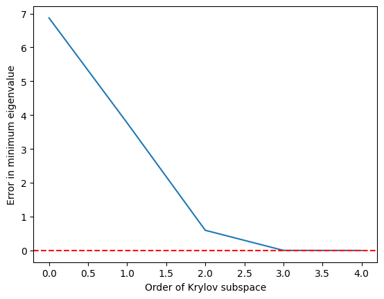
We see that the minimum eigenvalue is reached fairly accurately once the Krylov subspace has grown to and is perfect by
2.2 Time scaling with matrix dimension
Let us convince ourselves that the Krylov method can be advantageous over exact numerical eigensolvers in the following way:
- Construct random matrices (not sparse, not the ideal application for KQD)
- Determine eigenvalues using two methods: directly using NumPy and using a Krylov subspace.
- We choose a cutoff for how precise our eigenvalues must be, before we accept the Krylov estimates.
- Compare the wall time required to solve in these two ways.
Caveats: As we will discuss in detail below, Krylov quantum diagonalization is best applied to operators whose matrix representations are sparse and/or can be written using a small number of groups of commuting Pauli operators. The random matrices we are using here do not fit that description. These are only useful in probing the scale at which classical Krylov methods might be useful. Secondly, in using the Krylov method we will calculate eigenvalues using many different-sized Krylov subspaces. We will report the time required for the minimum-dimension Krylov subspace that achieves our required accuracy for the ground state eigenvalue. Again, this is a bit different from solving a problem that is intractable for exact eigensolvers, since we are using the exact solution to assess the dimension needed.
We begin by generating our set of random matrices.
import numpy as np

# Set the random seed
np.random.seed(42)

# how many random matrices will we make
num_matrix = 200

matrices = []
for m in range(1, num_matrix):
    matrices.append(np.random.rand(m, m))
We now diagonalize each matrix directly, using numpy. We calculate the time required for diagonalization for later comparison.
matrix_numpy_times = []
matrix_numpy_eigs = []
for mm in range(num_matrix - 1):
    t0 = time_mus()
    matrix_numpy_eigs.append(min(np.linalg.eig(matrices[mm]).eigenvalues))
    matrix_numpy_times.append(time_mus() - t0)

plt.plot(matrix_numpy_times)
plt.xlabel("Dimension of matrix")  # Add x-axis label
plt.ylabel("Time to diagonalize (microsec)")  # Add y-axis label
plt.show()
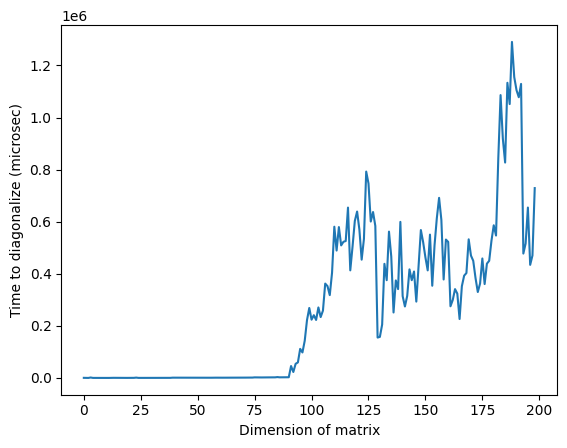
Note that in the image above, the anomalously high time around a dimension of 125 may be due to the random nature of the matrices or due to implementation on the classical processor used, but it is not reproducible. Re-running the code will yield a different profile with different anomalous peaks.
Now for each matrix we will build up a Krylov subspace and calculate eigenvalues in steps. At each step, we will check to see if the lowest eigenvalue has been obtained to within our specified absolute error. The subspace that first gives us eigenvalues within our specified error is the subspace for which we will record computation times. Executing this cell may take several minutes, depending on processor speed. Feel free to skip evaluation or reduce the maximum dimension of matrices diagonalized. Looking at the pre-calculated results is sufficient.
# Choose the absolute error you can tolerate, and make a list for tracking the Krylov subspace size
# at which that error is achieved.
abserr = 0.05
accept_subspace_size = []

# Lists to store total time spent on the Krylov method, and the subset of that time spent on
# diagonalizing the projected matrix.
matrix_krylov_tot_times = []
matrix_krylov_dim = []

# Step through all our random matrices
for mm in range(0, num_matrix - 1):
    test_ks, test_Hs, test_eigs, test_k_tot_times = krylov_full_build(
        np.ones(len(matrices[mm])), matrices[mm]
    )
    # We have not yet found a Krylov subspace that produces our minimum eigenvalue to
    # within the required error.
    found = 0
    for j in range(0, len(matrices[mm]) - 1):
        # If we still haven't found the desired subspace...
        if found == 0:
            # ...but if this one satisfies the requirement, then record everything
            if (
                abs((min(test_eigs[j]) - matrix_numpy_eigs[mm]) / matrix_numpy_eigs[mm])
                < abserr
            ):
                accept_subspace_size.append(j)
                matrix_krylov_tot_times.append(test_k_tot_times[j])
                matrix_krylov_dim.append(mm)
                found = 1
Let us plot the times we have obtained for these two methods for comparison:
plt.plot(matrix_numpy_times, color="blue")
plt.plot(matrix_krylov_dim, matrix_krylov_tot_times, color="green")
plt.xlabel("Dimension of matrix")  # Add x-axis label
plt.ylabel("Time to diagonalize (microsec)")  # Add y-axis label
plt.show()

These are the actual times required, but for the purposes of discussion, let us smooth these curves by averaging over a few adjacent points / matrix dimensions. This is done below:
smooth_numpy_times = []
smooth_krylov_times = []

# Choose the number of adjacent points over which to average forward;
# the same will be used backward.
smooth_steps = 10

# We will do this smoothing for all points/matrix dimensions
for i in range(len(matrix_krylov_tot_times)):
    # Ensure we don't exceed the boundaries of our lists
    start = max(0, i - smooth_steps)
    end = min(len(matrix_krylov_tot_times) - 1, i + smooth_steps)

    # Dummy variables for accumulating an average over adjacent points. This is done for both Krylov
    # and the NumPy calculations.
    smooth_count = 0
    smooth_numpy_sum = 0
    smooth_krylov_sum = 0

    for j in range(start, end):
        smooth_numpy_sum = smooth_numpy_sum + matrix_numpy_times[j]
        smooth_krylov_sum = smooth_krylov_sum + matrix_krylov_tot_times[j]
        smooth_count = smooth_count + 1

    # Appending the averaged adjacent values to our new smooth lists
    smooth_numpy_times.append(smooth_numpy_sum / smooth_count)
    smooth_krylov_times.append(smooth_krylov_sum / smooth_count)
plt.plot(smooth_numpy_times, color="blue")
plt.plot(smooth_krylov_times, color="green")
plt.xlabel("Dimension of matrix")  # Add x-axis label
plt.ylabel("Time to diagonalize (smoothed, microsec)")  # Add y-axis label
plt.show()

Note that the time required for the building of a Krylov subspace initially exceeds the time required for numpy's full diagonalization. But as the size of the matrix grows, the Krylov method becomes advantageous. This is true even if we lower our acceptable error, but the advantage sets in at a larger matrix size. This is worth picking apart.
The time complexity of numerical diagonalization is (with some variation among algorithms). The time complexity of generating an orthonormal basis of vectors is also . So the advantage of the Krylov method is not related to the use of orthonormal basis, but to the use of a particular orthonormal basis that effectively picks out the eigenvalues of interest. We have already seen this from the sketch of a proof in the first section of this lesson, and this is critical for the convergence guarantees in Krylov methods. Let us review our progress so far:
- For very large matrices, the Krylov subspace method may yield approximate eigenvalues within required tolerances faster than traditional diagonalization algorithms.
- For such very large matrices, the generation of a Krylov subspace is the most time-consuming part of the Krylov subspace method.
- Thus an efficient way of generating a Krylov subspace would be highly valuable. This is finally where quantum computer comes into the picture.
Check your understanding
Refer to the smoothed plot of diagonalization times versus matrix dimension above.
(a) At approximately what matrix dimension did the Krylov method become faster, according to this plot?
(b) What aspects of the calculation could change that dimension at which the Krylov method becomes faster?
Answer
(a) Answers may vary if you re-run the calculation, but the Krylov method becomes faster at approximately dimension 80-85.
(b) There are many possible answers. Some important factors are the precision we require and the sparsity of the matrices being diagonalized.
3. Krylov via time evolution
Everything that we have described so far can be done classically. So how and when would we use a quantum computer? For very large matrices, the Krylov method can require long computing times and large amounts of memory. The time required for matrix operation of on scales like in the worst case. Even multiplying sparse matrices on a vector (the typical case for classical Krylov-type solvers) has a time complexity scaling like . This is done for every vector we want in our subspace. The subspace dimension is usually not a significant fraction of , and often scales like . So generating all vectors scales like in the worst case. Although there are other steps, like orthogonalization, this is the dominant scaling to keep in mind.
Quantum computing allows us to change what attributes of the problem determine the scaling of the time and resources required. Instead of dependence on matrix size across the board, we will see things like number of shots and number of non-commuting Pauli terms that make up the Hamiltonian. Let’s explore how this works.
3.1 Time evolution
Recall that the operator that time-evolves a quantum state is (and it is very common, especially in quantum computing to drop the from the notation). One way of understanding and even realizing such an exponential function of an operator is to look at its Taylor series expansion. Note that this operation acting on some initial vector yields a sum of terms with increasing powers of applied to the initial state. It looks like we can just make our Krylov subspace by time-evolving our initial guess state!
The caveat is in realizing the time evolution on a real quantum computer. Many of the terms in the Hamiltonian will not commute with each other. So while some simple exponential operators like correspond to simple circuits, general Hamiltonians do not. And since they contain non-commuting terms, we can’t simply decompose the exponential into a product of simple ones, the way we can with numbers.
So this is not trivial, but this is a well-studied process in quantum computing. We carry out time-evolution on quantum computers using a process called trotterization, which in itself is a rich subject[10]. But at a very high level, by breaking the time evolution into very small steps, say steps of size , we limit the effects of the non-commutativity of terms.
where .
Let us call a Krylov subspace of order r that we generated in the classical context using powers of H directly a “power Krylov subspace”.
Now we generate a similar space using the unitary time-evolution operator ; we'll refer to this as the “unitary Krylov space” . The power Krylov subspace that we use classically cannot be generated directly on a quantum computer as is not a unitary operator. Using the unitary Krylov subspace can be shown to give similar convergence guarantees as the power Krylov subspace, namely, the ground state error converges efficiently as long as the initial state has overlap with the true ground state that is not exponentially vanishing, and as long as there is a sufficient gap between eigenvalues. See Ref [1] for a more precise discussion of convergence.
Here, powers of become different time steps (the power of is stepping forward by a time ). We can label the element of the subspace that is time-evolved for total time as .
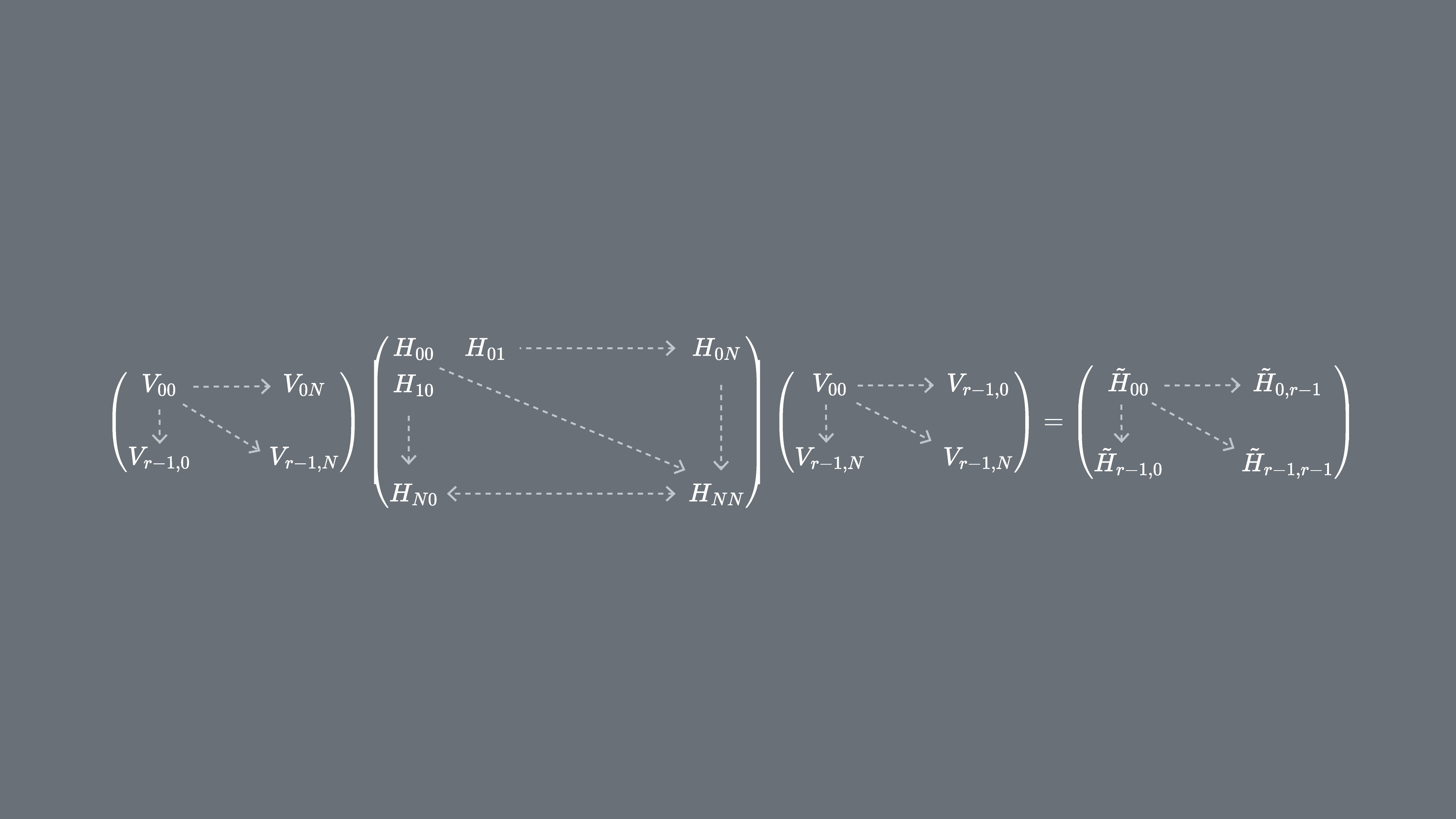
We can project our Hamiltonian H on to the unitary Krylov subspace, . In other words, we calculate each matrix element of in the basis. We'll refer to this projected matrix as .
3.2 How to implement on a quantum computer
The matrix elements of are given by the expectation values , which can be estimated using the quantum computer. Keep in mind that can be written as a sum of Pauli operators on different qubits, and that not all the Pauli operators can be measured simultaneously. We can sort the Pauli terms into groups of commuting terms, and measure all those at once. But we may need many such groups to cover all the terms. So the number of distinct commuting groups into which the terms can be partitioned, becomes important.
Here is a Pauli string of the form or a set of such Pauli strings that commute with one another. Given that we can write as such a sum of measureable operators, the following expressions for matrix elements of can be realized using the Qiskit Runtime primitive Estimator.
Where are the vectors of the unitary Krylov space and are the multiples of the time step chosen. On a quantum computer, the calculation of each matrix elements can be done with any algorithm which allows us to obtain overlap between quantum states. In this lesson we'll focus on the Hadamard test. Given that the has dimension , the Hamiltonian projected into the subspace will have dimensions . With small enough (generally is sufficient to obtain convergence of estimates of eigenvalues) we can then easily diagonalize the projected Hamiltonian classically. However, we cannot directly diagonalize because of the non-orthogonality of the Krylov space vectors. We'll have to measure their overlaps and construct a matrix
This allows us to solve the eigenvalue problem in a non-orthogonal space (also called generalized eigenvalue problem)
One can then obtain estimates of the eigenvalues and eigenstates of by looking at the solutions of this generalized eigenvalue problem. For example, the estimate of the ground state energy is obtained by taking the smallest eigenvalue and the ground state from the corresponding eigenvector . The coefficients in determines the contribution of the different vectors that span .
Generalized eigenvalue problem
Why can we not simply diagonalize ? Since contains the information about the geometry of the Krylov basis (which is nonorthogonal in all but very special cases), on its own does not describe a projection of the full Hamiltonian, so its eigenvalues have no particular relation to those of the full Hamiltonian -- they could be any random values. Solving the generalized eigenvalue problem is required to obtain the approximate eigenvalues and eigenvectors corresponding to the projection of the full Hamiltonian into the Krylov space..
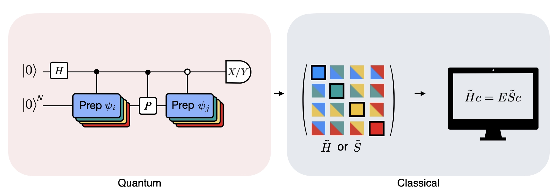
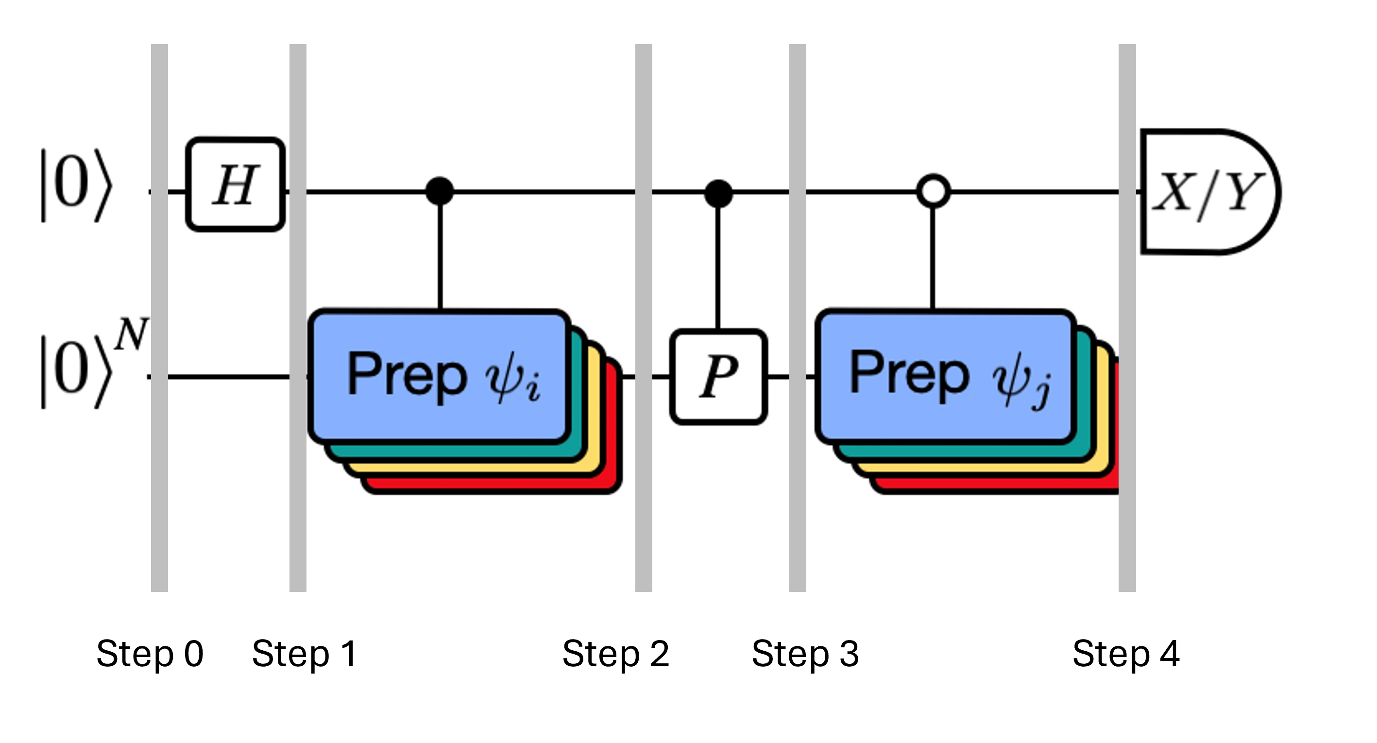
The Figure shows a circuit representation of the modified Hadamard test, a method that is used to compute the overlap between different quantum states. For each matrix element , a Hadamard test between the state , is carried out. This is highlighted in the figure by the color scheme for the matrix elements and the corresponding , operations. Thus, a set of Hadamard tests for all the possible combinations of Krylov space vectors is required to compute all the matrix elements of the projected Hamiltonian . The top wire in the Hadamard test circuit is an ancilla qubit which is measured either in the X or Y basis, its expectation value determines the value of the overlap between the states. The bottom wire represents all the qubits of the system Hamiltonian. The operation prepares the system qubit in the state controlled by the state of the ancilla qubit (similarly for ) and the operation represents Pauli decomposition of the system Hamiltonian . The implementation of this is on a quantum computer is shown in greater detail below.
4. Krylov quantum diagonalization on a quantum computer
We will now implement Krylov quantum diagonalization on a real quantum computer. Let's start by importing some useful packages.
import numpy as np
import scipy as sp
import matplotlib.pylab as plt
from typing import Union, List
import warnings

from qiskit.quantum_info import SparsePauliOp, Pauli
from qiskit.circuit import Parameter
from qiskit import QuantumCircuit, QuantumRegister
from qiskit.circuit.library import PauliEvolutionGate
from qiskit.synthesis import LieTrotter

# from qiskit.providers.fake_provider import Fake20QV1
from qiskit_ibm_runtime import QiskitRuntimeService, EstimatorV2 as Estimator, Batch

import itertools as it

warnings.filterwarnings("ignore")
We define the function below to solve the generalized eigenvalue problem we just explained above.
def solve_regularized_gen_eig(
    h: np.ndarray,
    s: np.ndarray,
    threshold: float,
    k: int = 1,
    return_dimn: bool = False,
) -> Union[float, List[float]]:
    """
    Method for solving the generalized eigenvalue problem with regularization

    Args:
        h (numpy.ndarray):
            The effective representation of the matrix in our Krylov subspace
        s (numpy.ndarray):
            The matrix of overlaps between vectors of our Krylov subspace
        threshold (float):
            Cut-off value for the eigenvalue of s
        k (int):
            Number of eigenvalues to return
        return_dimn (bool):
            Whether to return the size of the regularized subspace

    Returns:
        lowest k-eigenvalue(s) that are the solution of the regularized generalized eigenvalue problem

    """
    s_vals, s_vecs = sp.linalg.eigh(s)
    s_vecs = s_vecs.T
    good_vecs = np.array([vec for val, vec in zip(s_vals, s_vecs) if val > threshold])
    h_reg = good_vecs.conj() @ h @ good_vecs.T
    s_reg = good_vecs.conj() @ s @ good_vecs.T
    if k == 1:
        if return_dimn:
            return sp.linalg.eigh(h_reg, s_reg)[0][0], len(good_vecs)
        else:
            return sp.linalg.eigh(h_reg, s_reg)[0][0]
    else:
        if return_dimn:
            return sp.linalg.eigh(h_reg, s_reg)[0][:k], len(good_vecs)
        else:
            return sp.linalg.eigh(h_reg, s_reg)[0][:k]
At least in initial benchmarking, it is useful to know an exact classical solution to check convergence behavior. The function below calculates the ground state energy of a Hamiltonian, using the Hamiltonian and the number of qubits as arguments.
def single_particle_gs(H_op, n_qubits):
    """
    Find the ground state of the single particle(excitation) sector
    """
    H_x = []
    for p, coeff in H_op.to_list():
        H_x.append(set([i for i, v in enumerate(Pauli(p).x) if v]))

    H_z = []
    for p, coeff in H_op.to_list():
        H_z.append(set([i for i, v in enumerate(Pauli(p).z) if v]))

    H_c = H_op.coeffs

    print("n_sys_qubits", n_qubits)

    n_exc = 1
    sub_dimn = int(sp.special.comb(n_qubits + 1, n_exc))
    print("n_exc", n_exc, ", subspace dimension", sub_dimn)

    few_particle_H = np.zeros((sub_dimn, sub_dimn), dtype=complex)

    sparse_vecs = [
        set(vec) for vec in it.combinations(range(n_qubits + 1), r=n_exc)
    ]  # list all of the possible sets of n_exc indices of 1s in n_exc-particle states

    m = 0
    for i, i_set in enumerate(sparse_vecs):
        for j, j_set in enumerate(sparse_vecs):
            m += 1

            if len(i_set.symmetric_difference(j_set)) <= 2:
                for p_x, p_z, coeff in zip(H_x, H_z, H_c):
                    if i_set.symmetric_difference(j_set) == p_x:
                        sgn = ((-1j) ** len(p_x.intersection(p_z))) * (
                            (-1) ** len(i_set.intersection(p_z))
                        )
                    else:
                        sgn = 0

                    few_particle_H[i, j] += sgn * coeff

    gs_en = min(np.linalg.eigvalsh(few_particle_H))
    print("single particle ground state energy: ", gs_en)
    return gs_en
4.1 Step 1: Map problem to quantum circuits and operators
Now we will define a Hamiltonian. This is distinct from the function above in that the function above takes a Hamiltonian as an argument and returns only the ground state, and it does so classically. This Hamiltonian we define here determines the energy levels of all energy eigenstates, and this Hamiltonian can be constructed using Pauli operators and implemented on a quantum computer.
We choose a Hamiltonian corresponding to a chain of spins which can have any orientation in space, called a "Heisenberg chain". We assume that the spin can be influenced by its nearest neighbors (the and spins) but not by more distant neighbors. We also allow for the possibility that the interaction between spins is different when the spins point along different axes. This asymmetry sometimes arises, for example, due to the structure of the crystal lattice into which spins are embedded.
# Define problem Hamiltonian.
n_qubits = 10
# coupling strength for XX, YY, and ZZ interactions
JX = 1
JY = 3
JZ = 2

# Define the Hamiltonian:
H_int = [["I"] * n_qubits for _ in range(3 * (n_qubits - 1))]
for i in range(n_qubits - 1):
    H_int[i][i] = "Z"
    H_int[i][i + 1] = "Z"
for i in range(n_qubits - 1):
    H_int[n_qubits - 1 + i][i] = "X"
    H_int[n_qubits - 1 + i][i + 1] = "X"
for i in range(n_qubits - 1):
    H_int[2 * (n_qubits - 1) + i][i] = "Y"
    H_int[2 * (n_qubits - 1) + i][i + 1] = "Y"
H_int = ["".join(term) for term in H_int]
H_tot = [
    (term, JZ)
    if term.count("Z") == 2
    else (term, JY)
    if term.count("Y") == 2
    else (term, JX)
    for term in H_int
]

# Get operator
H_op = SparsePauliOp.from_list(H_tot)
print(H_tot)
[('ZZIIIIIIII', 2), ('IZZIIIIIII', 2), ('IIZZIIIIII', 2), ('IIIZZIIIII', 2), ('IIIIZZIIII', 2), ('IIIIIZZIII', 2), ('IIIIIIZZII', 2), ('IIIIIIIZZI', 2), ('IIIIIIIIZZ', 2), ('XXIIIIIIII', 1), ('IXXIIIIIII', 1), ('IIXXIIIIII', 1), ('IIIXXIIIII', 1), ('IIIIXXIIII', 1), ('IIIIIXXIII', 1), ('IIIIIIXXII', 1), ('IIIIIIIXXI', 1), ('IIIIIIIIXX', 1), ('YYIIIIIIII', 3), ('IYYIIIIIII', 3), ('IIYYIIIIII', 3), ('IIIYYIIIII', 3), ('IIIIYYIIII', 3), ('IIIIIYYIII', 3), ('IIIIIIYYII', 3), ('IIIIIIIYYI', 3), ('IIIIIIIIYY', 3)]
The code below restricts the Hamiltonian to single particle states, and uses the spectral norm to set a good size for our time step . We heuristically choose a value for the time-step dt (based on upper bounds on the Hamiltonian norm). Ref [9] showed that a sufficiently small timestep is , and that it is preferable up to a point to underestimate this value rather than overestimate, since overestimating can allow contributions from high-energy states to corrupt even the optimal state in the Krylov space. On the other hand, choosing to be too small leads to worse conditioning of the Krylov subspace, since the Krylov basis vectors differ less from timestep to timestep.
# Get Hamiltonian restricted to single-particle states
single_particle_H = np.zeros((n_qubits, n_qubits))
for i in range(n_qubits):
    for j in range(i + 1):
        for p, coeff in H_op.to_list():
            p_x = Pauli(p).x
            p_z = Pauli(p).z
            if all(p_x[k] == ((i == k) + (j == k)) % 2 for k in range(n_qubits)):
                sgn = ((-1j) ** sum(p_z[k] and p_x[k] for k in range(n_qubits))) * (
                    (-1) ** p_z[i]
                )
            else:
                sgn = 0
            single_particle_H[i, j] += sgn * coeff
for i in range(n_qubits):
    for j in range(i + 1, n_qubits):
        single_particle_H[i, j] = np.conj(single_particle_H[j, i])

# Set dt according to spectral norm
dt = np.pi / np.linalg.norm(single_particle_H, ord=2)
dt
np.float64(0.17453292519943295)
We specify the number of Trotter steps to use in the time evolution. We also specify a maximum Krylov dimension of 4. This Krylov dimension is not large enough for realistic applications. But it is sufficient for this example. Furthermore, we will check for convergence at even smaller dimensions. We will explore methods in later lessons that allow us to scale and project our Hamiltonians onto larger subspaces.
# Set parameters for quantum Krylov algorithm
krylov_dim = 4  # size of krylov subspace
num_trotter_steps = 4
dt_circ = dt / num_trotter_steps
State preparation
Pick a reference state that has some overlap with the ground state. For this Hamiltonian, We use the a state with an excitation in the middle qubit as our reference state.
qc_state_prep = QuantumCircuit(n_qubits)
qc_state_prep.x(int(n_qubits / 2) + 1)
qc_state_prep.draw("mpl", scale=0.5)

Time evolution
We can realize the time-evolution operator generated by a given Hamiltonian: via the Lie-Trotter approximation. For simplicity we use the built-in PauliEvolutionGate in the time-evolution circuit. The general syntax for this is this.
t = Parameter("t")

## Create the time-evo op circuit
evol_gate = PauliEvolutionGate(
    H_op, time=t, synthesis=LieTrotter(reps=num_trotter_steps)
)

qr = QuantumRegister(n_qubits)
qc_evol = QuantumCircuit(qr)
qc_evol.append(evol_gate, qargs=qr)
<qiskit.circuit.instructionset.InstructionSet at 0x7ccaa4664250>
We will use a version of this below in the Hadamard test, but stepping forward for times .
Hadamard test
Recall that we wish to calculate the matrix elements of both and the Gram matrix using the Hadamard test. Let's review how this works in this context, focusing first on the construction of The overall process is depicted graphically below. The layers of colored state preparation blocks serve as a reminder that this process is carried out for all combinations of and in our subspace.
The states of the system at the steps indicated are:
Here is a Pauli term in the decomposition of the Hamiltonian (note that it cannot be a linear combination of multiple commuting Pauli terms since that would not be unitary -- grouping is possible using a different construction we will show later) , are controlled operations that prepare , vectors of the unitary Krylov space, with . Applying measurements of and to this circuit calculates the real and imaginary parts, respectively, of the matrix elements we require.
Starting from Step 4 above, apply the Hadamard gate to the zeroth qubit.
Then measure either or .
From the identity . Similarly, measuring yields
Adding these steps to the time-evolution we set up previously we write the following.
## Create the time-evo op circuit
evol_gate = PauliEvolutionGate(
    H_op, time=dt, synthesis=LieTrotter(reps=num_trotter_steps)
)

## Create the time-evo op dagger circuit
evol_gate_d = PauliEvolutionGate(
    H_op, time=dt, synthesis=LieTrotter(reps=num_trotter_steps)
)
evol_gate_d = evol_gate_d.inverse()

# Put pieces together
qc_reg = QuantumRegister(n_qubits)
qc_temp = QuantumCircuit(qc_reg)
qc_temp.compose(qc_state_prep, inplace=True)
for _ in range(num_trotter_steps):
    qc_temp.append(evol_gate, qargs=qc_reg)
for _ in range(num_trotter_steps):
    qc_temp.append(evol_gate_d, qargs=qc_reg)
qc_temp.compose(qc_state_prep.inverse(), inplace=True)

# Create controlled version of the circuit
controlled_U = qc_temp.to_gate().control(1)

# Create hadamard test circuit for real part
qr = QuantumRegister(n_qubits + 1)
qc_real = QuantumCircuit(qr)
qc_real.h(0)
qc_real.append(controlled_U, list(range(n_qubits + 1)))
qc_real.h(0)

print("Circuit for calculating the real part of the overlap in S via Hadamard test")
qc_real.draw("mpl", fold=-1, scale=0.5)
Circuit for calculating the real part of the overlap in S via Hadamard test

We warned already about the depth involved in Trotter circuits. Performing the Hadamard test in these conditions can yield an even deeper circuit, especially once we decompose to native gates. This will increase even more if we account for the topology of the device. So before using any time on the quantum computer, it is a good idea to check the 2-qubit depth of our circuit.
print(
    "Number of layers of 2Q operations",
    qc_real.decompose(reps=2).depth(lambda x: x[0].num_qubits == 2),
)
Number of layers of 2Q operations 14401
A circuit of this depth cannot return usable results on modern quantum computers. If we are to construct and we need a better way. This is the reason for the efficient Hadamard test introduced below.
4. 2 Step 2. Optimize circuits and operators for target hardware
Efficient Hadamard test
We can optimize the deep circuits for the Hadamard test that we have obtained by introducing some approximations and relying on some assumption about the model Hamiltonian. For example, consider the following circuit for the Hadamard test:
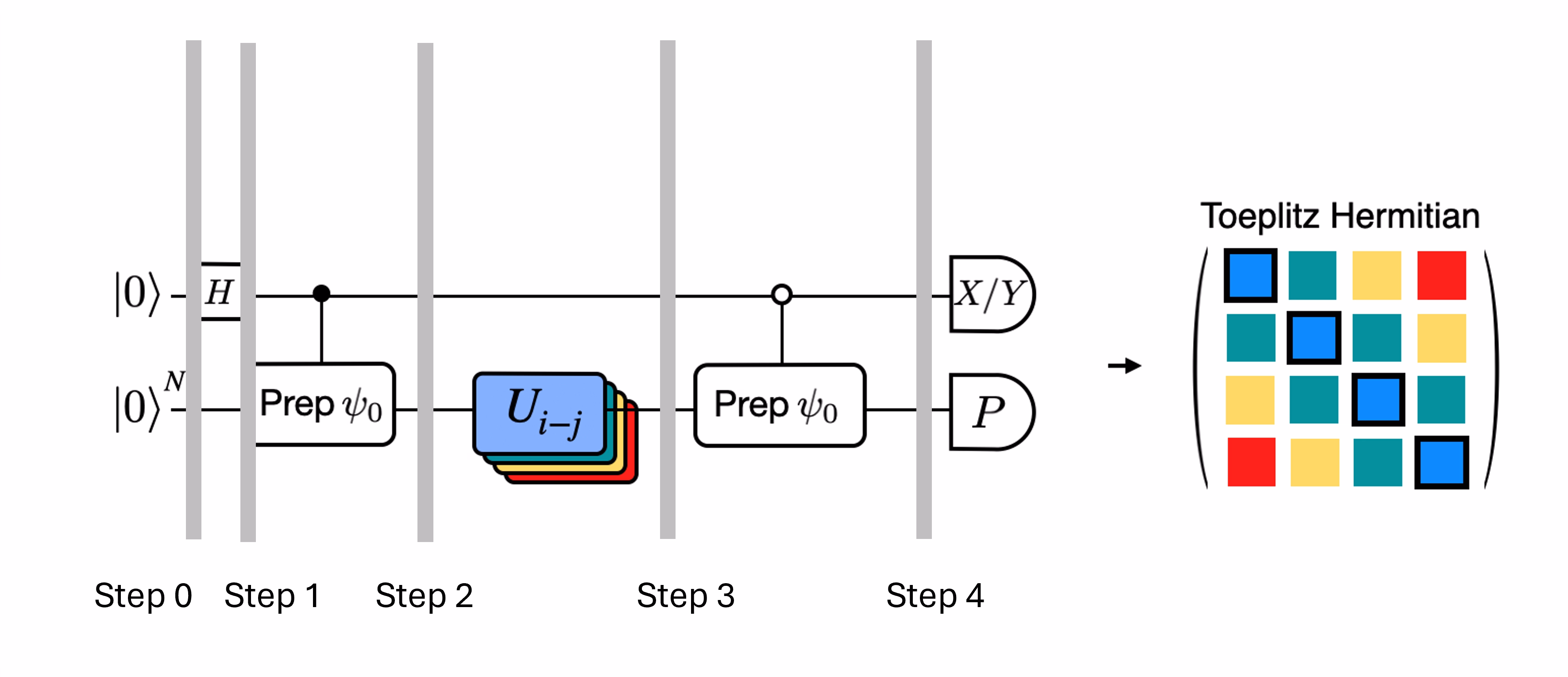
Assume we can classically calculate , the eigenvalue of under the Hamiltonian . This is satisfied when the Hamiltonian preserves the U(1) symmetry. Although this may seem like a strong assumption, there are many cases where it is safe to assume that there is a vacuum state (in this case it maps to the state) which is unaffected by the action of the Hamiltonian. This is true for example for chemistry Hamiltonians that describe stable molecule (where the number of electrons is conserved). Given that the gate , prepares the desired reference state , for example, to prepare the HF state for chemistry would be a product of single-qubit NOTs, so controlled- is just a product of CNOTs. Then the circuit above implements the following state prior to measurement:
where we have used the classical simulable phase shift from step 2 to 3. Therefore the expectation values are
Using these assumptions we were able to write the expectation values of operators of interest with fewer controlled operations. In fact, we only need to implement the controlled state preparation and not controlled time evolutions. Reframing our calculation as above will allow us to greatly reduce the depth of the resulting circuits.
Note that as a bonus, since the Pauli operator now appears as a measurement at the end of the circuit rather than as a controlled gate in the middle, it can be measured alongside other commuting Pauli operators as in the decomposition given above.
Decompose time-evolution operator with Trotter decomposition
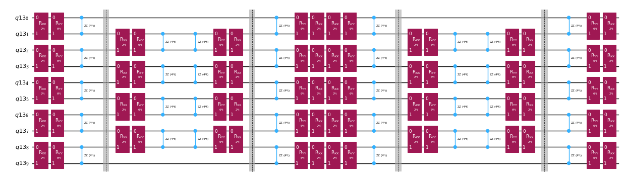
Instead of implementing the time-evolution operator exactly we can use the Trotter decomposition to implement an approximation of it. Repeating several times a certain order Trotter decomposition gives us further reduction of the error introduced from the approximation. In the following, we directly build the Trotter implementation in the most efficient way for the interaction graph of the Hamiltonian we are considering (nearest neighbor interactions only). In practice we insert Pauli rotations , , with coupling strengths and and a parametrized angle , which correspond to the approximate implementation of . Given the difference in definition of the Pauli rotations and the time-evolution that we are trying to implement, we'll have to use the parameter to achieve a time-evolution of . Furthermore, we reverse the order of the operations for odd number of repetitions of the Trotter steps, which is functionally equivalent but allows for synthesizing adjacent operations in a single unitary. This gives a much shallower circuit than what is obtained using the generic PauliEvolutionGate() functionality.
t = Parameter("t")

# Create instruction for rotation about XX+YY-ZZ:
Rxyz_circ = QuantumCircuit(2)
Rxyz_circ.rxx(2 * JX * t, 0, 1)
Rxyz_circ.ryy(2 * JY * t, 0, 1)
Rxyz_circ.rzz(2 * JZ * t, 0, 1)
Rxyz_instr = Rxyz_circ.to_instruction(label="R J_x XX + J_y YY + J_z ZZ")

interaction_list = [
    [[i, i + 1] for i in range(0, n_qubits - 1, 2)],
    [[i, i + 1] for i in range(1, n_qubits - 1, 2)],
]  # linear chain

qr = QuantumRegister(n_qubits)
trotter_step_circ = QuantumCircuit(qr)
for i, color in enumerate(interaction_list):
    for interaction in color:
        trotter_step_circ.append(Rxyz_instr, interaction)
    if i < len(interaction_list) - 1:
        trotter_step_circ.barrier()
reverse_trotter_step_circ = trotter_step_circ.reverse_ops()

qc_evol = QuantumCircuit(qr)
for step in range(num_trotter_steps):
    if step % 2 == 0:
        qc_evol = qc_evol.compose(trotter_step_circ)
    else:
        qc_evol = qc_evol.compose(reverse_trotter_step_circ)

qc_evol.decompose().draw("mpl", fold=-1, scale=0.5)
We prepare an initial state again for this efficient Hadamard test.
control = 0
excitation = int(n_qubits / 2) + 1
controlled_state_prep = QuantumCircuit(n_qubits + 1)
controlled_state_prep.cx(control, excitation)
controlled_state_prep.draw("mpl", fold=-1, scale=0.5)

Template circuits for calculating matrix elements of and via Hadamard test
The only difference between the circuits used in the Hadamard test will be the phase in the time-evolution operator and the observables measured. Therefore we can prepare a template circuit which represent the generic circuit for the Hadamard test, with placeholders for the gates that depend on the time-evolution operator.
# Parameters for the template circuits
parameters = []
for idx in range(1, krylov_dim):
    parameters.append(dt_circ * (idx))
# Create modified hadamard test circuit
qr = QuantumRegister(n_qubits + 1)
qc = QuantumCircuit(qr)
qc.h(0)
qc.compose(controlled_state_prep, list(range(n_qubits + 1)), inplace=True)
qc.barrier()
qc.compose(qc_evol, list(range(1, n_qubits + 1)), inplace=True)
qc.barrier()
qc.x(0)
qc.compose(controlled_state_prep.inverse(), list(range(n_qubits + 1)), inplace=True)
qc.x(0)

qc.decompose().draw("mpl", fold=-1)
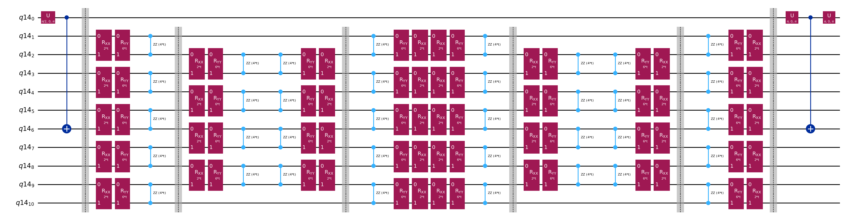
print(
    "The optimized circuit has 2Q gates depth: ",
    qc.decompose().decompose().depth(lambda x: x[0].num_qubits == 2),
)
The optimized circuit has 2Q gates depth: 50
This depth is substantially reduced compared to the original Hadamard test. This depth is manageable on modern quantum computers, though it is still quite high. We will need to use state-of-the-art error mitigation to obtain useful results.
Select a backend on which to run our quantum Krylov calculation, so that we can transpile our circuit for running on that quantum computer.
# Use the least-busy backend or specify a quantum computer using the syntax commented out below.
service = QiskitRuntimeService()
backend = service.least_busy(operational=True, simulator=False)

# Or you may choose a specify backend and channel if necessary for your workflow.
# service = QiskitRuntimeService(channel="ibm_quantum_platform")
# backend = service.backend("ibm_fez")
We now transpile our circuits and operators.
from qiskit.transpiler.preset_passmanagers import generate_preset_pass_manager

target = backend.target
basis_gates = list(target.operation_names)
pm = generate_preset_pass_manager(
    optimization_level=3, backend=backend, basis_gates=basis_gates
)

qc_trans = pm.run(qc)
print(qc_trans.depth(lambda x: x[0].num_qubits == 2))
print(qc_trans.count_ops())
qc_trans.draw("mpl", fold=-1, idle_wires=False, scale=0.5)
36
OrderedDict([('rz', 410), ('sx', 361), ('cz', 156), ('x', 18), ('barrier', 6)])

After optimization, our transpiled two-qubit depth is further reduced.
4.3 Step 3. Execute using a Qiskit Runtime primitive
We now create PUBs for execution with Estimator.
# Define observables to measure for S
observable_S_real = "I" * (n_qubits) + "X"
observable_S_imag = "I" * (n_qubits) + "Y"

observable_op_real = SparsePauliOp(
    observable_S_real
)  # define a sparse pauli operator for the observable
observable_op_imag = SparsePauliOp(observable_S_imag)

layout = qc_trans.layout  # get layout of transpiled circuit
observable_op_real = observable_op_real.apply_layout(
    layout
)  # apply physical layout to the observable
observable_op_imag = observable_op_imag.apply_layout(layout)
observable_S_real = (
    observable_op_real.paulis.to_labels()
)  # get the label of the physical observable
observable_S_imag = observable_op_imag.paulis.to_labels()

observables_S = [[observable_S_real], [observable_S_imag]]

# Define observables to measure for H
# Hamiltonian terms to measure
observable_list = []
for pauli, coeff in zip(H_op.paulis, H_op.coeffs):
    # print(pauli)
    observable_H_real = pauli[::-1].to_label() + "X"
    observable_H_imag = pauli[::-1].to_label() + "Y"
    observable_list.append([observable_H_real])
    observable_list.append([observable_H_imag])

layout = qc_trans.layout

observable_trans_list = []
for observable in observable_list:
    observable_op = SparsePauliOp(observable)
    observable_op = observable_op.apply_layout(layout)
    observable_trans_list.append([observable_op.paulis.to_labels()])

observables_H = observable_trans_list

# Define a sweep over parameter values
params = np.vstack(parameters).T

# Estimate the expectation value for all combinations of
# observables and parameter values, where the pub result will have
# shape (# observables, # parameter values).
pub = (qc_trans, observables_S + observables_H, params)
Circuits for are classically calculable. We carry this out before moving on to the case using a quantum computer.
from qiskit.quantum_info import StabilizerState, Pauli

qc_cliff = qc.assign_parameters({t: 0})

# Get expectation values from experiment
S_expval_real = StabilizerState(qc_cliff).expectation_value(
    Pauli("I" * (n_qubits) + "X")
)
S_expval_imag = StabilizerState(qc_cliff).expectation_value(
    Pauli("I" * (n_qubits) + "Y")
)

# Get expectation values
S_expval = S_expval_real + 1j * S_expval_imag

H_expval = 0
for obs_idx, (pauli, coeff) in enumerate(zip(H_op.paulis, H_op.coeffs)):
    # Get expectation values from experiment
    expval_real = StabilizerState(qc_cliff).expectation_value(
        Pauli(pauli[::-1].to_label() + "X")
    )
    expval_imag = StabilizerState(qc_cliff).expectation_value(
        Pauli(pauli[::-1].to_label() + "Y")
    )
    expval = expval_real + 1j * expval_imag

    # Fill-in matrix elements
    H_expval += coeff * expval

print(H_expval)
(10+0j)
Although we were able to reduce our gate depth by orders of magnitude using the efficient Hadamard test, the depth is still sufficient to require state-of-the-art error mitigation. Below, we specify attributes of the mitigation being used. All of the methods used are important, but it is worth called out probabilistic error amplification (PEA) specifically. This powerful technique comes with a great deal of quantum overhead. The calculation done here can take 20 minutes or more to run on a real quantum computer. You may wish to play with the parameters below to increase or decrease precision and consequentially overhead. The default settings below yield high-fidelity results.
# Experiment options
num_randomizations = 300
num_randomizations_learning = 20
max_batch_circuits = 20
shots_per_randomization = 100
learning_pair_depths = [0, 4, 24]
noise_factors = [1, 1.3, 1.6]

# Base option formatting
options = {
    # Builtin resilience settings for ZNE
    "resilience": {
        "measure_mitigation": True,
        "zne_mitigation": True,
        "zne": {"noise_factors": noise_factors},
        # TREX noise learning configuration
        "measure_noise_learning": {
            "num_randomizations": num_randomizations_learning,
            "shots_per_randomization": shots_per_randomization,
        },
        # PEA noise model configuration
        "layer_noise_learning": {
            "max_layers_to_learn": 10,
            "layer_pair_depths": learning_pair_depths,
            "shots_per_randomization": shots_per_randomization,
            "num_randomizations": num_randomizations_learning,
        },
    },
    # Randomization configuration
    "twirling": {
        "num_randomizations": num_randomizations,
        "shots_per_randomization": shots_per_randomization,
        "strategy": "all",
    },
    # Experimental settings for PEA method
    "experimental": {
        # # Just in case, disable any further qiskit transpilation not related to twirling / DD
        # "skip_transpilation": True,
        # Execution configuration
        "execution": {
            "max_pubs_per_batch_job": max_batch_circuits,
            "fast_parametric_update": True,
        },
        # Error Mitigation configuration
        "resilience": {
            # ZNE Configuration
            "zne": {
                "amplifier": "pea",
                "return_all_extrapolated": True,
                "return_unextrapolated": True,
                "extrapolated_noise_factors": [0] + noise_factors,
            }
        },
    },
}
Finally, we execute the circuits for and with Estimator.
# This job required 17 minutes of QPU time to run on a Heron r2 processor. This is only an estimate.
# Your execution time may vary.

with Batch(backend=backend) as batch:
    # Estimator
    estimator = Estimator(mode=batch, options=options)

    job = estimator.run([pub], precision=1)
4.4 Step 4. Post-process and analyze results
What we have obtained from the quantum computer are the individual matrix elements of and the commuting Pauli groups that make up the matrix elements of . These terms must be combined to recover our matrices, so that we can solve the generalized eigenvalue problem.
# Store the outputs as 'results'.
results = job.result()[0]
Calculate Effective Hamiltonian and Overlap matrices
First calculate the phase accumulated by the state during the uncontrolled time evolution
prefactors = [
    np.exp(-1j * sum([c for p, c in H_op.to_list() if "Z" in p]) * i * dt)
    for i in range(1, krylov_dim)
]
Once we have the results of the circuit executions we can post-process the data to calculate the matrix elements of
# Assemble S, the overlap matrix of dimension D:
S_first_row = np.zeros(krylov_dim, dtype=complex)
S_first_row[0] = 1 + 0j

# Add in ancilla-only measurements:
for i in range(krylov_dim - 1):
    # Get expectation values from experiment
    expval_real = results.data.evs[0][0][i]  # automatic extrapolated evs if ZNE is used
    expval_imag = results.data.evs[1][0][i]  # automatic extrapolated evs if ZNE is used

    # Get expectation values
    expval = expval_real + 1j * expval_imag
    S_first_row[i + 1] += prefactors[i] * expval

S_first_row_list = S_first_row.tolist()  # for saving purposes

S_circ = np.zeros((krylov_dim, krylov_dim), dtype=complex)

# Distribute entries from first row across matrix:
for i, j in it.product(range(krylov_dim), repeat=2):
    if i >= j:
        S_circ[j, i] = S_first_row[i - j]
    else:
        S_circ[j, i] = np.conj(S_first_row[j - i])
from sympy import Matrix

Matrix(S_circ)
And the matrix elements of
import itertools

# Assemble S, the overlap matrix of dimension D:
H_first_row = np.zeros(krylov_dim, dtype=complex)
H_first_row[0] = H_expval

for obs_idx, (pauli, coeff) in enumerate(zip(H_op.paulis, H_op.coeffs)):
    # Add in ancilla-only measurements:
    for i in range(krylov_dim - 1):
        # Get expectation values from experiment
        expval_real = results.data.evs[2 + 2 * obs_idx][0][
            i
        ]  # automatic extrapolated evs if ZNE is used
        expval_imag = results.data.evs[2 + 2 * obs_idx + 1][0][
            i
        ]  # automatic extrapolated evs if ZNE is used

        # Get expectation values
        expval = expval_real + 1j * expval_imag
        H_first_row[i + 1] += prefactors[i] * coeff * expval

H_first_row_list = H_first_row.tolist()

H_eff_circ = np.zeros((krylov_dim, krylov_dim), dtype=complex)

# Distribute entries from first row across matrix:
for i, j in itertools.product(range(krylov_dim), repeat=2):
    if i >= j:
        H_eff_circ[j, i] = H_first_row[i - j]
    else:
        H_eff_circ[j, i] = np.conj(H_first_row[j - i])
from sympy import Matrix

Matrix(H_eff_circ)
Finally, we can solve the generalized eigenvalue problem for :
and get an estimate of the ground state energy
gnd_en_circ_est_list = []
for d in range(1, krylov_dim + 1):
# Solve generalized eigenvalue problem
gnd_en_circ_est = solve_regularized_gen_eig(
H_eff_circ[:d, :d], S_circ[:d, :d], threshold=1e-1
)
gnd_en_circ_est_list.append(gnd_en_circ_est)
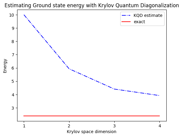
print("The estimated ground state energy is: ", gnd_en_circ_est)
The estimated ground state energy is:  10.0
The estimated ground state energy is:  5.933953916292923
The estimated ground state energy is:  4.4101773995740645
The estimated ground state energy is:  3.921288588521255
For a single-particle sector, we can efficiently calculate the ground state of this sector of the Hamiltonian classically
gs_en = single_particle_gs(H_op, n_qubits)
n_sys_qubits 10
n_exc 1 , subspace dimension 11
single particle ground state energy:  2.391547869638771
len(H_op)
27
plt.plot(
    range(1, krylov_dim + 1),
    gnd_en_circ_est_list,
    color="blue",
    linestyle="-.",
    label="KQD estimate",
)
plt.plot(
    range(1, krylov_dim + 1),
    [gs_en] * krylov_dim,
    color="red",
    linestyle="-",
    label="exact",
)
plt.xticks(range(1, krylov_dim + 1), range(1, krylov_dim + 1))
plt.legend()
plt.xlabel("Krylov space dimension")
plt.ylabel("Energy")
plt.title("Estimating Ground state energy with Krylov Quantum Diagonalization")
plt.show()
5. Discussion and extension
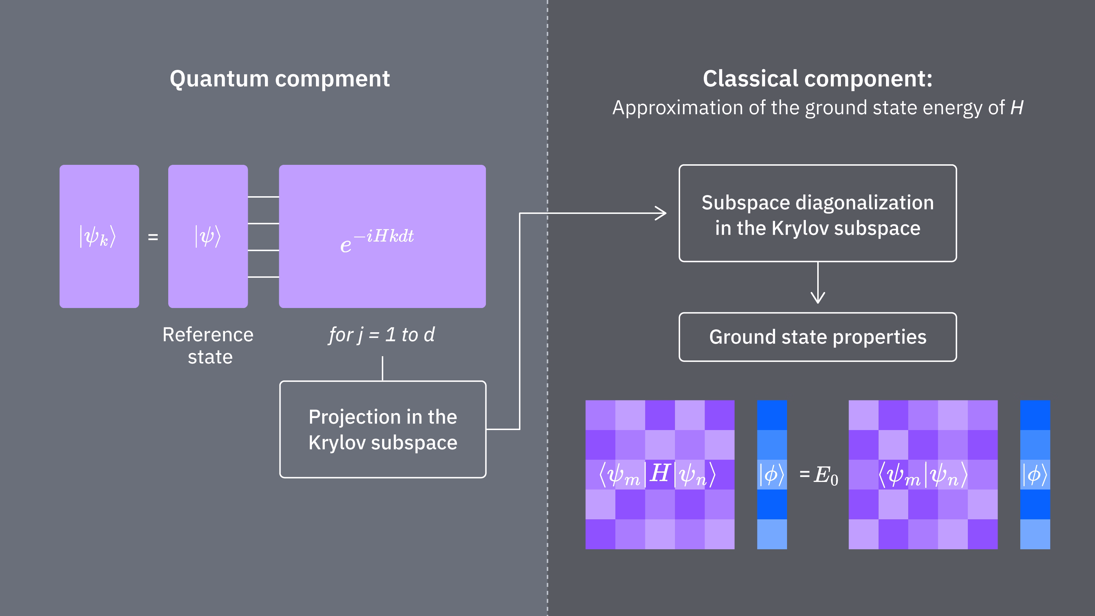
To recap, we start with a reference state, then evolve it for different periods of time to generate the unitary Krylov subspace. We project our Hamiltonian onto that subspace. We also estimate the overlaps of the subspace vectors. Finally we solve the lower-dimensional, generalized eigenvalue problem classically.
Let’s compare what determines computational costs of using the Krylov technique classically and quantum mechanically. There are not perfect analogs between classical and quantum approaches for all steps. This table collects some scaling of different steps for consideration.
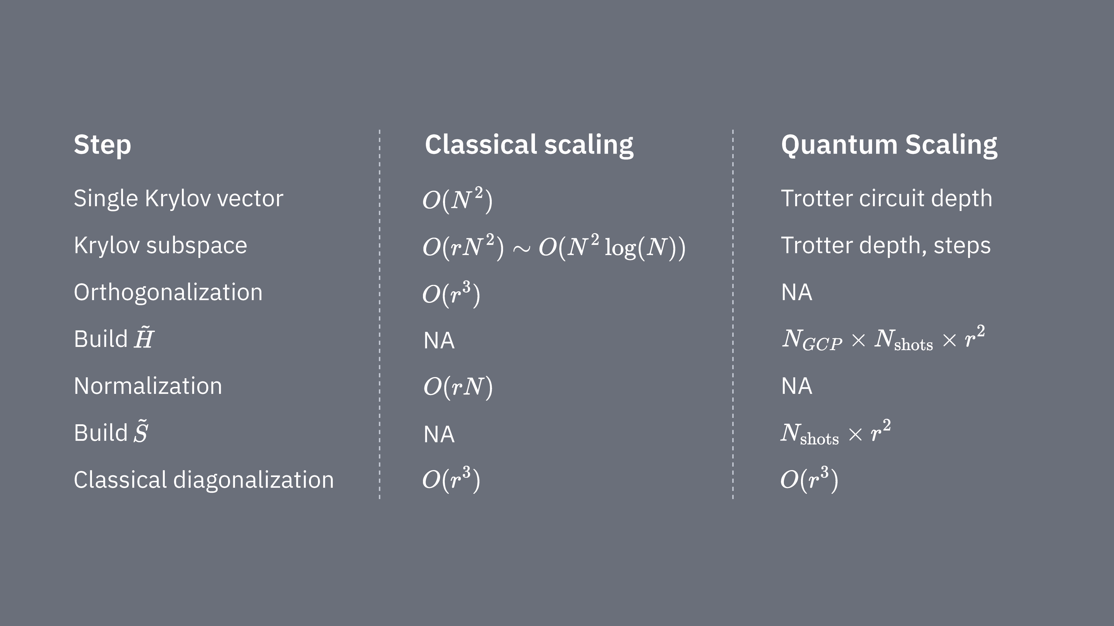
Recall that Hamiltonians generally have terms that cannot be simultaneously measured (because they do not commute with on another). We sort terms in the Hamiltonian into groups of commuting Pauli operators that can all be measured simultaneously, and we may require many such groups to account for all the terms that do not commute with one another. To build up on a quantum computer requires separate measurements for each group of commuting Pauli strings in the Hamiltonian, and each of those requires many shots. We must do this for different matrix elements, corresponding to combinations of different time evolution factors. There are sometimes ways to reduce this, but in this rough treatment, the time required for this scales like The elements of must be estimated, which scales like . Finally, solving the generalized eigenvalue problem in the projected space, classically, takes
We see that quantum Krylov diagonalization may be useful in cases where the number of commuting Pauli groups in the Hamiltonian is relatively small. These scaling dependencies suggest some applications where the Krylov method can be useful, and others where it likely will not be. Some Hamiltonians have high complexity when mapped to qubits, involving many non-commuting Pauli strings that cannot easily be partitioned into a few commuting groups. This is often true of quantum chemistry problems, for example. This complexity presents two primary challenges for near-term quantum computers:
- The estimation of each element of becomes computationally expensive due to the large number of terms.
- The required Trotter circuits become prohibitively deep.
Both of the above points will be less problematic when quantum computers reach fault-tolerance, but they must be considered in the near term. Even systems with “simpler” mappings than those in quantum chemistry may experience the same impediments, if the Hamiltonians have too many non-commuting terms. The Krylov method is most useful where the Hamiltonian can be partitioned into relatively few commuting Pauli groups, and where is easy to implement in trotter circuits. Both of these conditions are satisfied, for example, for many lattice models of interest in physics. KQD is especially useful if very little is known about the ground state. This stems from its inherent convergence guarantees and its applicability in scenarios where alternative methods are untenable due to insufficient ground state knowledge.
While KQD is a powerful tool, the protocol's time-consuming aspects, particularly the estimation of each element of the projected Hamiltonian and the overlap of Krylov states, represent opportunities for improvement. An alternative approach involves leveraging Krylov methods in conjunction with sampling-based methods, which are the subject of the next lesson.
6. Appendices
Appendix I: Krylov subspace from real time-evolutions
The unitary Krylov space is defined as
for some timestep that we will determine later. Temporarily assume is even: then define . Notice that when we project the Hamiltonian into the Krylov space above, it is indistinguishable from the Krylov space
that is, where all the time-evolutions are shifted backward by timesteps. The reason it is indistinguishable is because the matrix elements
are invariant under overall shifts of the evolution time, since the time-evolutions commute with the Hamiltonian. For odd , we can use the analysis for .
We want to show that somewhere in this Krylov space, there is guaranteed to be a low-energy state. We do so by way of the following result, which is derived from Theorem 3.1 in [3]:
Claim 1: there exists a function such that for energies in the spectral range of the Hamiltonian (that is, between the ground state energy and the maximum energy)...
- for all values of that lie away from , that is, it is exponentially suppressed
- is a linear combination of for
We give a proof below, but that can be safely skipped unless one wants to understand the full, rigorous argument. For now we focus on the implications of the above claim. By property 3 above, we can see that the shifted Krylov space above contains the state . This is our low-energy state. To see why, write in the energy eigenbasis:
where is the kth energy eigenstate and is its amplitude in the initial state . Expressed in terms of this, is given by
using the fact that we can replace by when it acts on the eigenstate . The energy error of this state is therefore
To turn this into an upper bound that is easier to understand, we first separate the sum in the numerator into terms with and terms with :
We can upper bound the first term by ,
where the first step follows because for every in the sum, and the second step follows because the sum in the numerator is a subset of the sum in the denominator. For the second term, first we lower bound the denominator by , since : adding everything back together, this gives
To simplify what is left, notice that for all these , by the definition of we know that . Additionally upper bounding and upper bounding gives
This holds for any , so if we set equal to our goal error, then the error bound above converges towards that exponentially with the Krylov dimension . Also note that if then the term actually goes away entirely in the above bound.
To complete the argument, we first note that the above is just the energy error of the particular state , rather than the energy error of the lowest energy state in the Krylov space. However, by the (Rayleigh-Ritz) variational principle, the energy error of the lowest energy state in the Krylov space is upper bounded by the energy error of any state in the Krylov space, so the above is also an upper bound on the energy error of the lowest energy state, that is, the output of the Krylov quantum diagonalization algorithm.
A similar analysis as the above can be carried out that additionally accounts for noise and the thresholding procedure discussed in the notebook. See [2] and [4] for this analysis.
Appendix II: proof of Claim 1
The following is mostly derived from [3], Theorem 3.1: let and let be the space of residual polynomials (polynomials whose value at 0 is 1) of degree at most . The solution to
is
and the corresponding minimal value is
We want to convert this into a function that can be expressed naturally in terms of complex exponentials, because those are the real time-evolutions that generate the quantum Krylov space. To do so, it is convenient to introduce the following transformation of energies within the spectral range of the Hamiltonian to numbers in the range : define
where is a timestep such that . Notice that and grows as moves away from .
Now using the polynomial with the parameters a, b, d set to , , and d = int(r/2), we define the function:
where is the ground state energy. We can see by inserting that is a trigonometric polynomial of degree , that is, a linear combination of for . Furthermore, from the definition of above we have that and for any in the spectral range such that we have
References:
[1] https://arxiv.org/abs/2407.14431
[2] https://arxiv.org/abs/1811.09025
[3] https://people.math.ethz.ch/~mhg/pub/biksm.pdf
[4] https://academic.oup.com/book/36426
[5] https://en.wikipedia.org/wiki/Krylov_subspace
[6] Krylov Subspace Methods: Principles and Analysis, Jörg Liesen, Zdenek Strakos https://academic.oup.com/book/36426
[7] Iterative Methods for Sparse Linear Systems" by Yousef Saad
[8] "MINRES-QLP: A Krylov Subspace Method for Indefinite or Singular Symmetric Systems" by Sou-Cheng Choi, Christopher Paige, and Michael Saunders (https://epubs.siam.org/doi/10.1137/100787921)
[9] Ethan N. Epperly, Lin Lin, and Yuji Nakatsukasa. "A theory of quantum subspace diagonalization". SIAM Journal on Matrix Analysis and Applications 43, 1263–1290 (2022).